Journal of Physical and Chemical Reference Data 26, 1125 (1997); https://doi.org/10.1063/1.555997 26, 1125
© 1997 American Institute of Physics and American Chemical Society.
A Formulation for the Static Permittivity
of Water and Steam at Temperatures from
238 K to 873 K at Pressures up to 1200 MPa,
Including Derivatives and Debye–Hückel
Coefficients
Cite as: Journal of Physical and Chemical Reference Data 26, 1125 (1997); https://
doi.org/10.1063/1.555997
Submitted: 12 February 1997 . Published Online: 15 October 2009
D. P. Fernández, A. R. H. Goodwin, Eric W. Lemmon, J. M. H. Levelt Sengers, and R. C. Williams
ARTICLES YOU MAY BE INTERESTED IN
The IAPWS Formulation 1995 for the Thermodynamic Properties of Ordinary Water Substance
for General and Scientific Use
Journal of Physical and Chemical Reference Data 31, 387 (2002); https://
doi.org/10.1063/1.1461829
A Database for the Static Dielectric Constant of Water and Steam
Journal of Physical and Chemical Reference Data 24, 33 (1995); https://
doi.org/10.1063/1.555977
The Dielectric Constant of Water and Debye-Hückel Limiting Law Slopes
Journal of Physical and Chemical Reference Data 19, 371 (1990); https://
doi.org/10.1063/1.555853

A Formulation for the Static Permittivity of Water and Steam
at Temperatures from 238 K to 873 K at Pressures up to 1200 MPa,
Including Derivatives and Debye–Hu
¨
ckel Coefficients
D. P. Ferna
´
ndez
a)
Physical and Chemical Properties Division, National Institute of Standards and Technology, Gaithersburg, Maryland 20899 and
Departamento Quı
´
mica de Reactores, Comisio
´
n Nacional de Energı
´
a Atomica, Avenue del Libertador 8250, 1429 Buenos Aires, Argentina
A. R. H. Goodwin and E. W. Lemmon
b)
Center for Applied Thermodynamics Studies, University of Idaho, Moscow, Idaho 83844-1011
J. M. H. Levelt Sengers
Physical and Chemical Properties Division, National Institute of Standards and Technology, Gaithersburg, Maryland 20899
R. C. Williams
Center for Applied Thermodynamics Studies, University of Idaho, Moscow, Idaho 83844-1011
Received February 12, 1997; revised manuscript received March 17, 1997
A new formulation is presented of the static relative permittivity or dielectric constant
of water and steam, including supercooled and supercritical states. The range is from
238 K to 873 K, at pressures up to 1200 MPa. The formulation is based on the ITS-90
temperature scale. It correlates a selected set of data from a recently published collection
of all experimental data. The set includes new data in the liquid water and the steam
regions that have not been part of earlier correlations. The physical basis for the formu-
lation is the so-called g-factor in the form proposed by Harris and Alder. An empirical
12-parameter form for the g-factor as a function of the independent variables temperature
and density is used. For the conversion of experimental pressures to densities, the newest
formulation of the equation of state of water on the ITS-90, prepared by Wagner and
Pruss, has been used. All experimental data are compared with the formulation. The
reliability of the new formulation is assessed in all subregions. Comparisons with previ-
ous formulations are presented. Auxiliary dielectric-constant formulations as functions of
temperature are included for the saturated vapor and liquid states. The pressure and
temperature derivatives of the dielectric constant and the Debye–Hu
¨
ckel limiting-law
slopes are calculated, their reliability is estimated, and they are compared with experi-
mentally derived values and with previous correlations. All equations are given in this
paper, along with short tables. An implementation of this formulation for the dielectric
constant is available on disk @A. H. Harvey, A. P. Peskin, and S. A. Klein, NIST/ASME
Steam Properties, NIST Standard Reference Database 10, Version 2.1, Standard Refer-
ence Data Program, NIST, Gaithersburg, MD ~1997!#.©1997 American Institute of
Physics and American Chemical Society. @S0047-2689~97!00104-9#
Key words: data correlation; Debye–Hu
¨
ckel coefficients; g-factor; ITS-90; static dielectric constant; static
relative permittivity; steam; supercritical steam; supercooled water; water.
Contents
1. Introduction................................ 1128
1.1. Importance............................. 1128
1.2. Complexity............................ 1128
1.3. Previous Correlations.................... 1129
1.4. Need for a New Correlation............... 1130
1.5. Choice of a Functional Form.............. 1130
1.6. Further Assumptions Made................ 1130
2. Physical Models............................ 1131
2.1. Dielectric Behavior of Polar, Polarizable
Dipolar Molecules....................... 1131
2.2. Statistical–Mechanical Theories of
Dielectrics............................. 1132
2.3. Theoretical and Phenomenological Estimates
a!
Present address: Facultad de Ciencias Exactas y Naturales, Universidad de
Buenos Aires, Ciudad Universitaria, Pabellon 2, 1428 Buenos Aires, Ar-
gentina.
b!
Present address: Physical and Chemical Properties Division, National In-
stitute of Standards and Technology, Boulder, CO 80303.
0047-2689/97/26(4)/1125/42/$14.00 J. Phys. Chem. Ref. Data, Vol. 26, No. 4, 1997
1125
for the g-Factor.........................
1133
3. Review of the Data......................... 1135
4. Correlation Procedure........................ 1136
4.1. Development of a Dielectric Constant
Equation for Water...................... 1136
4.2. Adaptive Regression Algorithm............ 1137
4.3. Equation of State for Water............... 1137
4.4. Weight Assignment...................... 1137
5. Results.................................... 1140
5.1. Results of the Regression Analysis......... 1140
5.2. Deviation Plots......................... 1140
5.3. Comparison with Previous Correlations...... 1145
5.4. Auxiliary Formulations for Saturated States.. 1146
5.5. Reliability Estimates in Various Regions.... 1146
5.6. Tabulation of the Dielectric Constant....... 1147
6. Derivatives of the Dielectric Constant.......... 1147
6.1. Derivatives Calculated from Experimental
Information............................ 1147
6.2. Derivatives from the Correlation........... 1148
6.3. Comparison of Derivatives from Experiment
and from Correlations.................... 1149
6.4. Reliability of the Derivatives of the
Dielectric Constant...................... 1153
7. Debye–Hu
¨
ckel Coefficients................... 1158
7.1. Definition and Values.................... 1158
7.2. Reliability............................. 1158
8. High-Temperature Behavior and Extrapolation. . . 1160
9. Conclusions................................ 1160
10. Acknowledgments.......................... 1161
11. Appendix.................................. 1161
12. References................................. 1165
List of Tables
1. Comparison of calculated and experimental
high-temperature values for the dielectric
constant of water........................... 1134
2. Initial absolute uncertainties assigned to the
static dielectric constant measurements from
each source based on Ref. 16................. 1136
3. Constants used in the dielectric constant
correlation................................. 1137
4. Values of the dielectric constant
e
at temperatures
T, pressures p, and densities
r
determined from
the equation of state, calculated g obtained
from Eq. ~16!, and final assigned weights....... 1138
5. Coefficients N
k
and exponents i
k
, j
k
and q of
Eq. ~34! for the g-factor..................... 1140
6. Dielectric constant data sources corresponding to
the symbols in the deviation plots. . ............ 1140
7. Comparison of previous formulations with the
present one ~H&K: Ref. 5; B&P: Ref. 10;
U&F: Ref. 11; A&W: Ref. 13!................ 1145
8. Coefficients L
i
and V
i
for Eqs. ~36! and ~37!.... 1146
9. Estimated absolute uncertainty of the predicted
dielectric constant, «
pred
at various state points. . . 1146
10. Values of (
]
e
/
]
T)
p
determined from the results
of Ferna
´
ndez et al. ~Ref. 16! with five methods
at p50.101325 MPa and at temperatures
between 273 K and 373 K.................... 1148
11. Values of (
]
2
e
/
]
T
2
)
p
determined from the
results of Ferna
´
ndez et al. ~Ref. 16! with
five methods at p50.101325 MPa and at
temperatures between 273 K and 373 K......... 1148
12. Predicted values of the dielectric constant, and
its first and second derivatives with respect to
pressure and temperature, at selected values of
temperature and pressure..................... 1149
13. First temperature derivative of the dielectric
constant at constant pressure.................. 1156
14. Second temperature derivative of the dielectric
constant at constant pressure.................. 1156
15. First pressure derivative of the dielectric
constant at constant temperature............... 1156
16. Second pressure derivative of the dielectric
constant at constant temperature............... 1157
17. Predicted values of the Debye–Hu
¨
ckel
coefficients at selected values of temperature and
pressure................................... 1157
18. Percentage difference of our predicted Debye–
Hu
¨
ckel coefficient values from those Archer and
Wang ~Ref. 13!............................. 1159
19. Dielectric constant of water and steam as a
function of temperature and pressure........... 1162
20. The dielectric constant of water and steam as a
function of temperature and density............ 1164
List of Figures
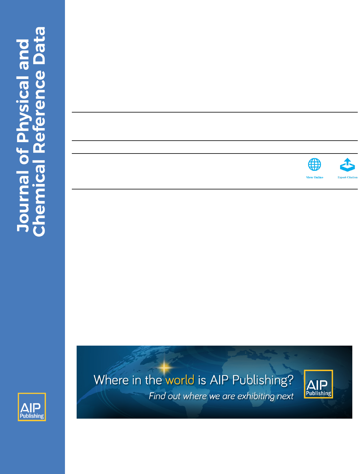
1. ~A! The evaluated experimental data for the
dielectric constant
e
of water and steam
~Ref. 3! above 400 K, in their dependence on
density and temperature. Isobars ~----!and
iso-
e
curves ~–•–•–! are indicated. Symbols:
Table 6....................................
~B!As Fig. 1~A!, but for the liquid region below
400 K. Symbols: Table 6..................... 1129
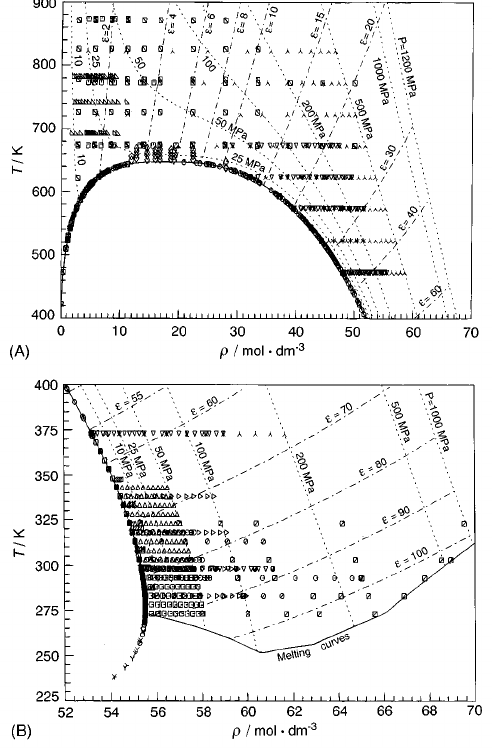
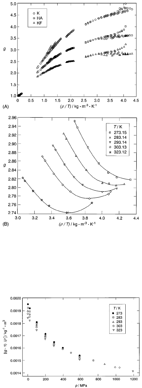
2. ~A! The Kirkwood g-factor
@
s#, modified to
include polarizability, Eq. ~15!, the Harris–
Alder ~Ref. 37! g-factor
@
h#, Eq. ~16!, and the
Kirkwood–Fro
¨
hlich ~Ref. 32! g-factor
@
D#,
Eq. ~19!, as functions of the variable
r
/T
for a subset of the data in Fig. 1. Symbols:
Table 6....................................
~B! The Harris–Alder g-factor for the
high-density Lees data ~Ref. 60! as a function of
r
/T...................................... 1135
3. Harris–Alder, Eq. ~16!, ~g21!/
r
versus pressure,
Lees data ~Ref. 60!.......................... 1135
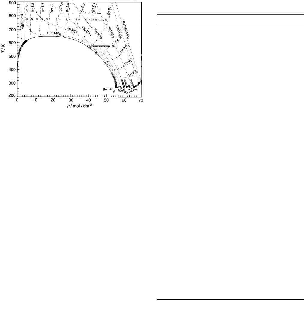
4. Location of the selected dielectric constant data
used in the correlation. Iso-g lines for the Harris–
Alder g-factor are indicated in the plot.
Symbols: Table 6........................... 1136
11261126 FERNANDEZ
ET AL.
J. Phys. Chem. Ref. Data, Vol. 26, No. 4, 1997
5. Deviations D
e
5
e
2
e
~calc.! of dielectric
constant
e
data from Eqs. ~21! and ~34!~and
coefficients listed in Table 5! for water at a
pressure of 0.101325 MPa and temperatures in
the range 235–373 K. Symbols: Table 6........ 1141
6. Deviations D
e
5
e
2
e
~calc.! of dielectric
constant
e
data from Eqs. ~21! and ~34!~with
coefficients listed in Table 5! for water at
temperatures between 238 K and 299 K. Symbols:
Table 6................................... 1142
7. Deviations D
e
5
e
2
e
~calc.! of dielectric
constant
e
data from Eqs. ~21! and ~34!~with
coefficients listed in Table 5! for water at
temperatures between 301 K and 338 K. Symbols:
Table 6................................... 1142
8. Deviations D
e
5
e
2
e
~calc.! of dielectric
constant
e
data from Eqs. ~21! and ~34!~with
coefficients listed in Table 5! for water at
temperatures between 343 K and 523 K. Symbols:
Table 6................................... 1143
9. Deviations D
e
5
e
2
e
~calc.! of dielectric
constant
e
data from Eqs. ~21! and ~34!~with
coefficients listed in Table 5! for water at
temperatures between 573 K and 743 K. Symbols:
Table 6................................... 1143
10. Deviations D
e
5
e
2
e
~calc.! of dielectric
constant
e
data from Eqs. ~21! and ~34!~with
coefficients listed in Table 5! for water at
temperatures between 773 K and 873 K. Symbols:
Table 6................................... 1144
11. Deviations D
e
5
e
2
e
~calc.! of dielectric
constant
e
data from Eqs. ~21! and ~34!~with
coefficients listed in Table 5! for saturated
liquid water and steam. Symbols: Table 6....... 1144
12. First derivative of the dielectric constant with
respect to pressure at constant temperature
(
]
e
/
]
p)
T
for water at temperatures between
273 K and 308 K. Symbols: Table 6;
‘‘experimental’’ values: 5-point Lagrangian
interpolation. Dashed curve: Ref. 13............ 1150
13. First derivative of the dielectric constant with
respect to pressure at constant temperature
(
]
e
/
]
p)
T
for water at temperatures between
313 K and 343 K. Symbols: Table 6;
‘‘experimental’’ values: 5-point Lagrangian
interpolation. Dashed curve: Ref. 13............ 1150
14. First derivative of the dielectric constant with
respect to pressure at constant temperature
(
]
e
/
]
p)
T
for water at temperatures between
373 K and 573 K. Symbols: Table 6;
‘‘experimental’’ values: 5-point Lagrangian
interpolation. Dashed curve: Ref. 13............ 1151
15. First derivative of the dielectric constant with
respect to pressure at constant temperature
(
]
e
/
]
p)
T
for water at temperatures between
623 K and 675 K. Symbols: Table 6;
‘‘experimental’’ values: 5-point Lagrangian
interpolation. Dashed curve: Ref. 13............ 1151
16. First derivative of the dielectric constant with
respect to pressure at constant temperature
(
]
e
/
]
p)
T
for water at temperatures between
723 K and 873 K. Symbols: Table 6;
‘‘experimental’’ values: 5-point Lagrangian
interpolation. Dashed curve: Ref. 13............ 1152
17. Departure from the formulation for the first
derivative of the dielectric constant with
respect to temperature at constant pressure
(
]
e
/
]
T)
p
for water at 0.101325 MPa in the range
of 235–373 K. Symbols: Table 6;
‘‘experimental’’ values: 5-point Lagrangian
interpolation. Dashed curve: Ref. 13............ 1153
18. First derivative of the dielectric constant with
respect to temperature at constant pressure
(
]
e
/
]
T)
p
for water at pressures between 0.1 MPa
and 25 MPa. Symbols: Table 6; ‘‘experimental’’
values: 5-point Lagrangian interpolation.
Dashed curve: Ref. 13....................... 1154
19. First derivative of the dielectric constant with
respect to temperature at constant pressure
(
]
e
/
]
T)
p
for water at pressures between 30 MPa
and 71 MPa. Symbols: Table 6; ‘‘experimental’’
values: 5-point Lagrangian interpolation.
Dashed curve: Ref. 13....................... 1154
20. First derivative of the dielectric constant with
respect to temperature at constant pressure
(
]
e
/
]
T)
p
for water at pressures between 75 MPa
and 297 MPa. Symbols: Table 6; ‘‘experimental’’
values: 5-point Lagrangian interpolation.
Dashed curve: Ref. 13....................... 1155
21. First derivative of the dielectric constant with
respect to temperature at constant pressure
(
]
e
/
]
T)
p
for water at pressures between
300 MPa and 595 MPa. Symbols: Table 6;
‘‘experimental’’ values: 5-point Lagrangian
interpolation. Dashed curve: Ref. 13............ 1155
22. The second temperature derivative of the
density, according to a variety of high-quality
equations of state....Ref. 100;----Ref.
101; full curve, Ref. 19; -•-•- Ref. 14.......... 1159
23. Comparison of high-temperature computer
simulation data for the SPC/E model with
our correlation. Isochores are for 1.0, 0.8, 0.6,
0.4, and 0.2 kg dm
2 3
, respectively, from top to
bottom. s, Wallqvist ~Ref. 58!; h , Mountain
~Ref. 58!; m, Neumann ~Ref. 57!; ! , simulated
coexistence curve, Guissani ~Ref. 56!; solid
curves: the present correlation................. 1160
List of Symbols
Roman
a radius of cavity
A
f
D.H. osmotic coefficient
A
V
D.H. coefficient for volume
A
H
D.H. coefficient for enthalpy
11271127A FORMULATION FOR THE STATIC PERMITTIVITY OF WATER AND STEAM
J. Phys. Chem. Ref. Data, Vol. 26, No. 4, 1997
A
K
D.H. coefficient for compressibility
A
C
D.H. coefficient for heat capacity
D.H. Debye–Hu
¨
ckel ~coefficient!
e unit vector
e charge of proton
E electric field
E
c
cavity field
E
o
external field
E
1
instantaneous local field
E
i
internal field or averaged local field
L
i
Lagrange-interpolation coefficients
M total dipole moment
n number density
N
A
Avogadro’s number
N
c
number of molecules inside a spherical cavity
N
k
coefficients in expression for g-factor
P dipolar density
P polarization per unit volume
p pressure
p
o
*
0.101 325 MPa
p(X
i
) weight factor for molecule i
q exponent for glass transition anomaly
T absolute temperature, ITS-90
T
c
critical temperature
U intermolecular energy
V
el
electrostatic energy
V
o
non-electrostatic energy
X
i
positional and orientational coordinates of mol-
ecule i
Greek
a
c
critical exponent
a
molecular polarizability
e
static dielectric constant or relative permittivity
e
o
permittivity of vacuum
e
`
infinite-frequency dielectric constant
u
reduced temperature difference with the critical
temperature
m
dipole moment for isolated molecule
m
d
effective dipole moment
n
refractive index
r
amount-of-substance density
r
c
critical density
1. Introduction
1.1. Importance
The dielectric properties of water in its fluid phases deter-
mine its solvent behavior in natural and industrial settings,
and its essential role in living organisms. One aspect of the
dielectric properties is the static ~zero-frequency limit! rela-
tive permittivity or dielectric constant. This property deter-
mines the strength of electrostatic interactions of ionic sol-
utes in water, and therefore plays a major role in aqueous
physical chemistry. In particular, the static dielectric constant
and its pressure and temperature derivatives determine the
infinite-dilution limiting slopes of thermodynamic properties
of electrolytes in water according to the theory of Debye and
Hu
¨
ckel,
1
and also play a key role in the Born model
2
of
solvation of aqueous electrolyte solutions. These values of
the dielectric constant and its derivatives can be derived in a
consistent way from a formulation of the static dielectric
constant of liquid water as a function of pressure and tem-
perature.
The temperature and pressure range of interest to geolo-
gists and geochemists far exceeds that of liquid water below
its boiling point. Pressurized high-temperature water, includ-
ing supercritical water, is encountered in the deep earth and
ocean. Furthermore, efficient generation of electricity by
means of steam requires reduction of shutdowns due to mal-
functioning. Knowledge of the fate and action of water im-
purities is of vital importance to the performance of boilers,
heat exchangers, and turbines. There is also a recent vigorous
interest in supercritical water as a reaction medium. In this
regime of strongly diverging compressibility, pressure is not
a useful independent variable, and formulations are conve-
niently done in terms of density and temperature as indepen-
dent variables.
1.2. Complexity
In what follows, the symbol
e
will denote the static rela-
tive permittivity or dielectric constant, made dimensionless
by expressing it in units of
e
o
, the vacuum permittivity.
The static dielectric constant
e
of water @Figs. 1~A!,1~B!#
has a complicated behavior not found in most other fluids.
In nonpolar fluids,
e
21 is roughly proportional to density,
with a prefactor depending on the molecular polarizability.
In polar fluids, the breaking of the correlations between the
dipoles as the temperature increases gives rise to a negative
temperature dependence of the dielectric constant at fixed
density.
This simple behavior is visible in water only in the dilute
steam phase. The actual behavior is dominated by the huge
increase of the dielectric constant in the region where water
is hydrogen-bonded. The experimental values of
e
range
from close to 1 in steam to over 100 in pressurized and
supercooled water.
The large rise of the dielectric constant in the range of
liquid and supercooled water has, so far, defied quantitative
theoretical description in terms of intermolecular forces, not-
withstanding valiant and sustained effort during the best part
of the present century. Computer simulations are beginning
to make inroads, but the results for the dielectric constant
appear to be highly sensitive to details of the intramolecular
and intermolecular potential, while any given potential can
usually give acceptable results only in limited ranges of tem-
perature and density. The high-temperature range is some-
what easier to describe, given the fact that hydrogen bonding
is much weaker. Promising results have been recently ob-
tained by computer simulation.
From the point of view of constructing an accurate corre-
lation, availability of theoretical guidance is desirable for
several reasons: it might suggest the form of a correlating
11281128 FERNANDEZ
ET AL.
J. Phys. Chem. Ref. Data, Vol. 26, No. 4, 1997
equation, could fill in data gaps, enable a choice between
discrepant data, and govern extrapolation. In Sec. 2, the
theory of the dielectric constant of a system of dipolar and
polarizable molecules is summarized, including the useful
models resulting from this theory, and high-temperature
computer simulation and analytical results are discussed and
referenced.
1.3. Previous Correlations
Quist and Marshall,
4
in 1965, produced an estimation of
the dielectric constant of water up to 1073 K in terms of the
Kirkwood equation, to be discussed in Sec. 2. Tabulated val-
ues of the density of water were used to convert pressure to
density. Values of
m
2
g were backed out from all available
data in the liquid up to 623 K and 1200 MPa, and fitted with
a function of density and pressure that contained four to five
adjustable parameters. There were no data available in the
supercritical regime at that time. Tabulated values were pre-
sented at temperatures up to 1073 K, at densities up to
1gcm
23
.
Helgeson and Kirkham,
5
in 1974, developed a correlation
of the dielectric constant of water up to high pressures and
temperatures for the purpose of developing the Born model
2
of solvation for aqueous solutions. This model characterizes
the water solvent solely by its dielectric constant. For
geochemical purposes it was important to extend the model
to supercritical states. These authors formulated the dielectric
constant itself as a polynomial in density and temperature
with 15 adjustable parameters. They fitted this function to
data of Oshry,
6
Owen et al.,
7
and Heger.
8
The latter data
extend into the supercritical regime. The range of the corre-
lation is up to 600 MPa and 773 K. The equation of state
used to convert pressure to density appears to have been that
of Keenan et al.
9
Pressure and temperature derivatives of the
dielectric constant were calculated and tabulated.
A correlation of the dielectric constant of water as a func-
tion of pressure and temperature was developed by Bradley
and Pitzer
10
in 1979. A somewhat different selection of data
in the liquid phase below 623 K was made than that of
Helgeson and Kirkham, and the Heger data were fitted in the
supercritical regime. The functional form chosen had nine
adjustable parameters. Debye–Hu
¨
ckel slopes were calculated
and tabulated for the range up to 623 K and 100 MPa.
Uematsu and Franck,
11
in 1980, recognized the need for a
formulation of the dielectric constant of water and steam that
would encompass the entire fluid region, including not only
the supercritical state but also the subcritical vapor. A key
role was played by the data of Heger et al., since pub-
lished.
12
The conversion from measured pressures to densi-
ties was achieved by means of the formulation for scientific
and general use ~IFC68! that was adopted by the Interna-
tional Association for the Properties of Steam in 1968. This
equation is now recognized to have shortcomings, and has
been supplanted by more recent high-quality formulations.
Uematsu and Franck included several data sets in the near-
and supercritical state that had not been considered before.
The dielectric constant was formulated as a polynomial in
density and inverse temperature, with ten adjustable param-
eters for the range up to 500 MPa and from 273 K to 823 K.
The emphasis of Uematsu and Franck was on the dielectric
constant in the supercritical regime. The issue of the deriva-
tives was not considered. At the low-temperature end in liq-
uid water, the temperature slope of the Uematsu–Franck cor-
relation is smaller in absolute value than the slope displayed
by most of the data.
A recent correlation of the static dielectric constant of all
fluid states of water is that of Archer and Wang
13
in 1990.
These authors used the relation proposed for the g-factor by
Kirkwood ~Sec. 2! as a starting point, and the high-quality
equation of state of Hill,
14
which we will denote as Hill90, to
convert pressure to density. They fit the quantity ~g2 1)/
r
.
Their fitting expression contains nine adjustable parameters
for the range from 238 K to 823 K up to ;500 MPa, includ-
ing data in supercooled water. The data available at pressures
FIG.1.~A!The evaluated experimental data for the dielectric constant
e
of
water and steam ~Ref. 3! above 400 K, in their dependence on density and
temperature. Isobars ~----!and iso-
e
curves ~– • – • –! are indicated.
Symbols: Table 6. ~B! As Fig. 1~A!, but for the liquid region below 400 K.
Symbols: Table 6.
11291129A FORMULATION FOR THE STATIC PERMITTIVITY OF WATER AND STEAM
J. Phys. Chem. Ref. Data, Vol. 26, No. 4, 1997
higher than 500 MPa were not included in the fit. The
Archer–Wang formulation has unusual features. First of all,
it uses not only density and temperature, but also pressure as
variables ~obviously not all independent!. Second, it uses
three anomalous terms that diverge strongly at a temperature
of 215 K ~well outside the range of available data!; this tem-
perature is also well below that of 228 K at which the com-
pressibility and viscosity diverge according to the analysis of
Angell and co-workers ~see Sec. 1.6!. The correlation of Ar-
cher and Wang gives an accurate representation of all dielec-
tric constant data known at the time, and includes a tabula-
tion of Debye–Hu
¨
ckel coefficients.
Johnson and Norton,
15
in a recent review, discuss the re-
lationship of the various formulations, and offer refinements
of the Helgeson and Kirkham and of the Uematsu and
Franck equations that reflect a better knowledge of critical
behavior and of the equation of state.
1.4. Need for a New Correlation
There are a number of reasons why it is desirable to revisit
the issue of the dielectric constant formulation. The first rea-
son is the availability of new experimental data in liquid
water.
16
For the first time, accurate data are available in the
steam phase,
17
see Ref. 3. Also, a vexing discrepancy be-
tween two groups of data sets in liquid water, reducing the
precision with which derivatives of the dielectric constant
and Debye–Hu
¨
ckel coefficients can be obtained, has been at
least partially resolved.
16
The second reason is the revision of the international tem-
perature scale to the ITS-90.
18
The Archer–Wang formula-
tion cannot be consistently adjusted to the new scale by a
simple shift of the temperature variable, because of the im-
plicit and explicit use of the Hill equation of state of water,
which is not on the new scale. The revision requires a new
formulation of the equation of state, which again is not a
matter of a simple shift of scale, since a variety of thermo-
dynamic data enters the formulation of the Helmholtz func-
tion from which the equation of state is derived. A new
Helmholtz function of water on ITS-90 has become available
since: that of Wagner and Pruss.
19
It has been adopted by the
International Association for the Properties of Water and
Steam.
20
Third, we considered it desirable to extend the formulation
over the full pressure range, up to 1190 MPa, for which data
are available, rather than cutting off at 500 MPa. Finally, we
considered the dependence on three variables, p, T, and
r
in
the formulation of the g-factor an undesirable feature, and
have decided not to use this approach.
1.5. Choice of Functional Form
We have experimented with many possible functional
forms for the correlation. An empirical polynomial in density
and temperature, as used by Uematsu and Franck, was cer-
tainly an option, and we performed some not completely
satisfactory fits with roughly ten adjustable parameters.
We have tried a 4-5 parameter dependence on the scaled
variable
r
/T, as suggested by Mulev et al.,
17
and found it
adequate for vapor and supercritical data, but not sufficiently
precise and flexible for the liquid phase.
Some previous correlations have been based on the
g-factor of Kirkwood ~Sec. 2!. It should be understood that
none of the existing correlations is based on a theoretical
expression for the Kirkwood g-factor. The expression is sim-
ply inverted, and values of g are calculated from the mea-
sured experimental data. The advantage of such a procedure
is that the g-factor varies only over a factor of 5 at most,
while the dielectric constant varies over 2 orders of magni-
tude.
We finally decided to correlate the dielectric constant by
means of the g-factor in the form proposed by Harris and
Alder ~see Sec. 2!. We do incorporate the known dipole mo-
ment and average polarizability of the isolated water mol-
ecule. The Harris–Alder g-factor is again treated as an em-
pirical property backed out from the experimental dielectric
constant data.
1.6. Further Assumptions Made
In the present formulation, possible anomalies of the di-
electric constant near the critical point have been ignored,
while that in the supercooled liquid has been accounted for
to some extent. As far as the latter anomaly is concerned, as
Speedy and Angell
21
have shown, many properties of super-
cooled water, such as compressibility and viscosity, appear
to diverge at a temperature of ;228 K.
Hodge and Angell
22
measured the dielectric constant of
emulsified supercooled water down to 238 K. This was a
very difficult experiment, because it is hard to avoid partial
crystallization of the water. The authors estimate the reliabil-
ity of their data as 2%. The data do agree well within this
uncertainty with other data that penetrate deeply into the
supercooled state.
23,24
Hodge and Angell fitted their data with a power law of the
form:
e
5 A
e
~
T/T
s
2 1
!
2 q
~1!
with q50.126, a weak divergence at most. Here T is the
temperature, and T
s
the glass transition temperature. Hodge
and Angell also fitted their data with a quadratic in tempera-
ture, measured in °C. In their Fig. 3, the quadratic appears
slightly too flat, missing the lowest-temperature point by
21%. The power-law expression, however, curves too
strongly, underestimating all points in the middle range by a
percent or more, and overshooting the lowest-temperature
point by a percent. We therefore considered the evidence for
a power-law divergence to be weak.
As a practical matter, however, we found that the Hodge
and Angell data are fitted better over the whole range when
one divergent term was used in addition to the set of regular
terms that defines the surface over most of the range. The
divergent term selected by our algorithm has a strong diver-
gence at 228 K, with an exponent of 21.2.
11301130 FERNANDEZ
ET AL.
J. Phys. Chem. Ref. Data, Vol. 26, No. 4, 1997

As far as the critical behavior of the dielectric constant is
concerned, it should be noted that in any formulation, such
as Refs. 4, 5, 11, and the present one, in which the leading
variation of the dielectric constant is proportional to the den-
sity, the strong critical divergence of the pressure and tem-
perature derivatives of the dielectric constant will be ~trivi-
ally! included. In the present formulation, the additional
subtle (12
a
c
)-type critical anomaly
e
5
e
c
1 A
~
12 T/T
c
!
12
a
c
, ~2!
which is expected to occur in the dielectric constant of
fluids
25,26
along the critical isochore, has not been included.
Here
a
c
is the critical exponent for the isochoric heat capac-
ity, the best estimate for its value being 0.11, a small number
characteristic of a weak anomaly; and
e
c
is the value of the
dielectric constant at the critical point. The anomalous term
is subtle, reaching a value of zero at the critical point, but
leading to a weak divergence of the first temperature deriva-
tive of the dielectric constant at constant volume. An
anomaly of this type has not been detected in the best ex-
periments in nonpolar pure fluids ~He, Ref. 27; SF
6
, Ref. 28;
Ne and N
2
, Ref. 29!, but it has been seen in CO, a weakly
polar fluid.
30
There is no theoretical prediction for the ampli-
tude of this anomaly in terms of the molecular dipole mo-
ment. The experimental dielectric constant data in near- and
supercritical steam are much too imprecise to allow an esti-
mate of the amplitude. Moreover, building into a formulation
the appropriate scaled behavior in terms of both density and
temperature is a nontrivial problem. For all these reasons, we
have decided not to incorporate the expected critical
anomaly into our formulation. The large size of the molecu-
lar dipole moment of water, however, is a warning that the
effect potentially could be substantial. Only new more accu-
rate measurements near the critical point of water could jus-
tify the introduction of a term reflecting the critical anomaly.
2. Physical Models
2.1. Dielectric Behavior of Polar, Polarizable
Dipolar Molecules
The first descriptions of the dielectric properties of mate-
rials were formulated in the 19th century. An example is the
well-known Clausius–Mossotti relation
e
2 1
e
1 2
5
n
a
3
e
0
~3!
for the dielectric constant
e
of a medium of number density
n5 N/V and molecular polarizability
a
. Lorentz
31
presented
a derivation of this equation by considering the internal field
E
i
, which acts on an individual polarizable molecule and
differs from the Maxwell field E inside the dielectric. The
Maxwell field E can be related to the external field E
0
for a
given shape of the dielectric. The dielectric constant is a
measure of the polarization P per unit volume induced by the
Maxwell field:
e
5 11
P
e
0
E
. ~4!
Lorentz
31
developed a procedure for calculating the internal
field by surrounding the molecule by a microscopic cavity, a
sphere large enough to contain many molecules, but outside
of which the medium can be replaced by a homogeneous
dielectric. The net effect of the external field on an empty
cavity inside the dielectric is to build up a polarization
charge on the cavity wall, which reduces the electric field
strength inside the cavity. In addition, Lorentz calculated the
contribution of the fields of the polarized molecules inside
the cavity to the internal field, found that it averaged to zero
for a distribution of the molecules on a regular lattice and
also for a completely random arrangement of the molecules,
and concluded that it could be set equal to zero. In both
cases, the Clausius–Mossotti relation, Eq. ~3!, results. In
fact, this proof is not valid
32
because it ignores the correla-
tion between the induced dipole moment on the molecule
considered and the polarization this dipole induces into sur-
rounding volume elements inside the cavity.
It was Debye
33
who, in the early part of this century, noted
that an important characteristic of dielectric materials was
not described by Eq. ~3!, namely the temperature dependence
of the dielectric constant found for many fluids. Debye pro-
posed that this feature is due to the presence of permanent
electric dipoles and he modified the Clausius–Mossotti equa-
tion by assuming that the same internal field that polarizes
the molecules also torques the dipoles. The result is
e
2 1
e
1 2
5
n
3
e
0
S
a
1
m
2
3kT
D
. ~5!
This linear relation of the dielectric constant and the inverse
temperature permits the extraction of the values of both the
molecular polarizability
a
and the dipole moment
m
from
experimental data for the temperature dependence of the di-
electric constant of a fluid.
Bell
32,34
calculated the interaction of a nonpolarizable
point dipole with its environment by considering it imbedded
in a molecular-size spherical cavity. The dipole polarizes its
environment, which produces a reaction field at the position
of the dipole; this reaction field adds to the dipole field.
Onsager
35
pointed out undesirable features in the Debye
equation, namely the prediction of the existence of a Curie
point below which a permanent electric moment exists not
found in real liquids. Also, the dipole moments derived by
Debye’s method from experimental data in high-dielectric
liquids are smaller than those found in the gas phase of the
same compound. Onsager traced these problems to the as-
sumption that the same internal field that polarizes the mol-
ecule also torques its dipole. In reality, the torquing or di-
recting field is smaller than the internal field. Onsager,
35
generalizing Bell’s method to the case of an external field
and a polarizable dipolar molecule, calculated the reaction
field due to polarization of the cavity wall. The reaction field
is parallel to the dipole and does not contribute to the torque.
It does enhance both the dipole moment and the induced
11311131A FORMULATION FOR THE STATIC PERMITTIVITY OF WATER AND STEAM
J. Phys. Chem. Ref. Data, Vol. 26, No. 4, 1997

moment, causing an effective dipole moment typically 20%–
40% larger, in common polar organic liquids, than that of the
isolated molecule.
Bo
¨
ttcher’s
32
form of Onsager’s equation for a pure fluid
consisting of polarizable dipoles is
~
e
2 1
!
~
2
e
1 1
!
9
e
5
n
e
0
S
a
*
1
~
m
*
!
2
3kT
D
,
a
*
/
a
5
m
*
/
m
5
~
n
2
12
!
~
2
e
1
n
2
!
~
2
e
11
!
3
, ~6!
a
5a
3
n
2
21
n
2
12
.
Here the symbol
n
stands for the refractive index of the
medium. Onsager introduced this quantity to eliminate both
the polarizability and the unspecified radius a of the cavity
from the expressions.
Bell’s and Onsager’s descriptions of the dielectric behav-
ior of dipolar fluids are mean-field theories in the sense that
an individual dipole is considered in interaction with a con-
tinuum. Considerable generalization is required for applica-
tion to the case of water, for which the molecules have strong
specific interactions. These generalizations are introduced in
Sec. 2.2.
2.2. Statistical–Mechanical Theories of Dielectrics
The statistical mechanical treatment of the dielectric be-
havior of a medium consisting of polar and/or polarizable
molecules, initiated by Kirkwood,
36
may be viewed as a gen-
eralization of the Lorentz approach in which only two limit-
ing cases, total order and total disorder, were assumed for the
molecules inside the cavity, and permanent dipoles were not
present.
In general, these statistical–mechanical theories
32
assume
that the polarization P is equal to the dipolar density P, and
neglect the influence of higher multipolar densities. For a
sample with volume V, the dipole density P is then related to
the statistical average of the instantaneous total dipole mo-
ment M,
^
M
&
,by
PV5
^
M
&
. ~7!
Equations ~4! and ~7! are the starting point for the micro-
scopic description of the static permittivity. The total inter-
molecular potential, including specific interactions such as
hydrogen bonding, can in principle be included in the calcu-
lation of the statistical average. With the external electric
field E
0
as the independent variable, Eqs. ~4! and ~7! result in
e
5 11
1
e
0
V
S
]
E
0
]
E
D
E50
S
]
]
E
0
^
M– e
&
D
E
0
5 0
, ~8!
where M is the total dipole moment vector and e is the unit
vector in the direction of the field. In Eq. ~8! only the linear
term in the power series expansions of P and M in powers of
E has been retained.
For special shapes of the dielectric, typically a sphere, the
internal field E can be straightforwardly related to the exter-
nal field E
0
. The total dipole moment M is composed of N
instantaneous molecular vectors, each of them made up from
permanent and induced parts. The induced dipole moment is
the product of a scalar polarizability and the instantaneous
local electric field E
l
at the position of the molecule. The
internal field E
i
is the average of the local field E
l
over time
and position of all molecules. The permanent dipole moment
is that of the isolated molecule. The average
^
M– e
&
,asa
function of E
o
, then has to be calculated as the average of
the sum of the instantaneous dipole moments of the N mol-
ecules. The total intermolecular energy U is included in the
Boltzmann factor for the statistical average. U is composed
of electrostatic, V
el
, as well as nonelectrostatic energies,
V
o
. The electrostatic energy, in this case, originates from
dipolar forces, with contributions from the potential energy
of the dipoles in the external field and in each other’s field,
and from polarization work required to bring the molecular
dipoles from the isolated-molecule value to the total value
including the induced contribution.
Because of the relatively short range of specific bonding
forces in liquids such as water, the Lorentz prescription, in
which only a number N
c
of molecules inside a spherical
cavity from the total number of molecules N is considered in
the average, should be a good approximation. The remaining
N2 N
c
molecules are replaced by a continuum of dielectric
constant
e
in which the spherical cavity is immersed. The
external field working on the sphere with N
c
molecules and
volume V is the cavity field E
c
,
E
o
5 E
c
5
3
e
2
e
1 1
E, ~9!
where E is the Maxwell field in the material outside the
sphere.
For a liquid composed of nonpolarizable molecules with
permanent dipole moment
m
one obtains
e
5 11
1
e
0
V
3
e
2
e
1 1
^
M
2
&
o
3kT
, ~10!
where M
2
5 M–M, M being now the sum of the dipole mo-
ments for the N
c
molecules inside the spherical cavity of
volume V.
^&
o
denotes the statistical average in the absence
of an external field. Equation ~10! is obtained by writing
V
el
in terms of E
o
, taking the derivative in Eq. ~8! and using
Eq. ~9!. The average
^
M
2
&
o
can be rewritten by defining the
Kirkwood
36
correlation factor g,
g5
1
u
m
u
2
E
p
~
X
i
!
m
i
–M
i
*
dX
i
, ~11!
where X
i
represents the positional and orientational coordi-
nates for the molecule i, and the weight factor p(X
i
) and the
average moment M
i
*
are defined according to
p
~
X
i
!
5
*
dX
N2i
exp
~
2 U/kT
!
*
dX
N
exp
~
2 U/kT
!
, ~12!
11321132 FERNANDEZ
ET AL.
J. Phys. Chem. Ref. Data, Vol. 26, No. 4, 1997

M
i
*
5
*
dX
N2i
M exp
~
2 U/kT
!
*
dX
N2i
exp
~
2 U/kT
!
, ~13!
where X
N2i
represent the positional and orientational coor-
dinates of the N
c
molecules, except for molecule i. With Eqs.
~11!–~13!, Eq. ~10! is rewritten as the so-called Kirkwood
equation
36
~
e
2 1
!
~
2
e
1 1
!
e
5
n
e
0
kT
g
m
2
, ~14!
where n5 N/V is the number density of the sample. The
quantity M
i
*
, given by Eq. ~13!, represents the average mo-
ment of the sphere containing N
c
molecules in the field of
the dipole of molecule i, held with fixed orientation. The
Kirkwood correlation factor g, given in Eq. ~11!, character-
izes the correlation between the molecular orientations due
to nondipolar interactions. Equation ~14! reduces to the On-
sager equation, Eq. ~6!, for nonpolarizable molecules
(
n
51! and for g5 1.
For polarizable molecules, the above definitions are no
longer valid. The induced moment depends on the local field
acting on molecule i,(E
1
)
i
, and is a function of the orien-
tations and positions of all other molecules. The average mo-
ment M
i
*
, given in Eq. ~13!, no longer depends on the co-
ordinates of molecule i alone. Kirkwood
36
explained that in
this case the dipole moment
m
is not that of the isolated
molecule because of the polarization of the molecule by its
neighbors, but no rigorous procedure was given to relate this
moment to that of the isolated molecule. Noting that the
contribution of the induced polarization to the dielectric con-
stant for polar polarizable fluids is in general small,
Kirkwood
36
supplemented Eq. ~14! with another term pro-
portional to the polarizability
a
:
~
e
2 1
!
~
2
e
1 1
!
3
e
5
n
e
0
S
a
1
1
3kT
g
m
2
D
. ~15!
This is only an approximate result for systems of polar po-
larizable molecules. Equation ~15! does not reduce to the
Clausius–Mossotti equation in the absence of a permanent
dipole. A different alternative was proposed by Harris and
Alder,
37
~
e
2 1
!
~
2
e
1 1
!
3
e
5
n
e
0
S
~
2
e
1 1
!
~
e
1 2
!
9
e
a
1
1
3kT
g
m
2
D
. ~16!
Equation ~16! does reduce to the Clausius–Mossotti for-
mula in the absence of a permanent dipole. It does not, how-
ever, reduce to the Onsager equation for g5 1. As in the case
of Eq. ~15!, the dipole moment
m
is not that of the isolated
molecule, and it is not possible to evaluate it without further
approximations. The procedure leading to Eq. ~16! was criti-
cized by various authors,
38,39
and others concurred with the
criticism.
40,41
The model conceived by Fro
¨
hlich
42
for a system of polar
polarizable molecules is a continuum with dielectric constant
e
`
in which molecules with dipole moment
m
d
and specific
nonelectrostatic interactions are immersed. The molecular di-
pole moment
m
d
is not that of the isolated molecule, but
includes that part of the induced dipole moment that arises
from the presence of permanent dipoles.
m
d
can be related to
the dipole moment
m
of the isolated molecule by
m
d
5
e
`
1 2
3
m
. ~17!
Again, a spherical cavity with N
c
molecules and volume V is
considered, now embedded in a continuum with dielectric
constant
e
`
. The external field working on this cavity is, in
this case,
E
o
5
3
e
2
e
1
e
`
E. ~18!
Finally, the Kirkwood–Fro
¨
hlich equation
32
is
~
e
2
e
`
!
~
2
e
1
e
`
!
e
~
e
`
1 2
!
2
5
1
9
n
e
0
kT
g
m
2
, ~19!
where g is the Kirkwood correlation factor of Eqs. ~11!, ~14!,
and ~15!. In the derivation of Eq. ~19! the contribution of the
induced polarization to the dielectric constant is rigorously
included for Fro
¨
hlich’s model, which is essentially Onsag-
er’s model with specific correlations added. The Kirkwood–
Fro
¨
hlich equation reduces to the Onsager equation for
g5 1.
The model of a continuum with dielectric constant
e
`
is a
mean-field theory and thus implies the neglect of the corre-
lations between the positions and the induced dipole moment
of the molecules.
32
As noticed by Hill,
40
Eq. ~19! is very
sensitive to the value selected for
e
`
. For instance, if the
value arising from dielectric relaxation measurements for liq-
uid water,
e
`
'4.5, is used together with the isolated-
molecule value for
m
, g values result unrealistically close to
unity. There are many different interpretations for
e
`
, asso-
ciated with the far-infrared dispersion of the water
molecule.
41,43,44
Repeatedly,
e
`
has been approximated by
the better known optical permittivity
e
`
5
n
2
, ~20!
where
n
is the refractive index.
In summary, the statistical–mechanical treatment of the
dielectric constant of water, a system of polar, polarizable
molecules with specific interactions, is a daunting problem
for which only approximate solutions are available at
present.
2.3. Theoretical and Phenomenological Estimates
for the
g
-Factor
The correlation factor g for water has been estimated on
the basis of a variety of models. The first value, g52.63 in
liquid water, was calculated by Oster and Kirkwood,
45
who
included only the contribution of first neighbors. Early mod-
els of ~a! bond-bending and ~b! bond-breaking assumed a
tetrahedral ice-I tridymite structure for the liquid phase, and
produced similar values for g, namely of 2.60 ~a! and 2.81
~b!, respectively, for liquid water at 273.15 K.
43
The bond-
11331133A FORMULATION FOR THE STATIC PERMITTIVITY OF WATER AND STEAM
J. Phys. Chem. Ref. Data, Vol. 26, No. 4, 1997

breaking model is able to reproduce the dielectric constant of
liquid water up to the critical point fairly well with only one
adjustable parameter.
For even higher temperatures, a break-up of the hydrogen
bonding network is expected. In this case, simpler models
may be appropiate to describe the static dielectric behavior
of the fluid. Franck et al.
46
used the linearized hypernetted-
chain analytic result for a collection of hard spheres with
embedded dipoles.
47
The equation obtained by Patey et al.
47
was fitted by Franck et al.
46
to experimental data at 673 K
and 823 K obtained by Heger
8,12
and by Deul.
48,49
The ef-
fective dipole moment, an adjustable parameter, was taken to
be 2.33 D. The authors presented
e
values for temperatures
up to 1273 K and densities up to 1000 kg m
2 3
~see Table 1!.
Goldman et al.
50
developed a second-order perturbation
theory for the Kirkwood correlation factor and obtained the
dielectric constant by means of a series expansion of the
dielectric constant in terms of the dipolar strength
m
2
r
/(3kT). They used the SPC/E intermolecular potential
for water.
51
This model consists of three-point, nonpolariz-
able rigid charges embedded in a Lennard-Jones core, with a
dipole moment of 2.35 D. Results were presented at tempera-
tures up to 1278 K and densities up to 1000 kg m
2 3
, and
showed good agreement with simulation values.
52
The values
obtained from the different theories for the average dipole
moment and the correlation factor g in the liquid can be
compared with those calculated with good accuracy for ice-
1h, namely
m
52.434 D and g5 3.00, respectively.
53
Table 1 shows the comparison of results obtained by
Goldman et al.
50
with the prediction of Franck et al.
46
and
with experimental data. The prediction by Franck et al. was
recalculated by us on the basis of Franck’s equation.
Much effort was recently expended in calculating the
static dielectric constant of liquid water by means of simula-
tion techniques,
52,54–57
The evaluation of the dipole correla-
tion is a time-consuming task, because an average has to be
obtained of the total instantaneous dipole moment of the en-
tire system. The actual values obtained for the static dielec-
tric constant have been found to be highly sensitive to details
of the intermolecular potential used. The most succesful in-
termolecular potential nowadays is the SPC/E,
51
by means of
which it has been possible to reproduce
e
along the coexist-
ence curve up to the critical point to within 10% of the ex-
perimental value.
55
For recent calculations with SPC/E, see
Ref. 57. For a critical intercomparison of all literature results
for SPC/E, and a comparison with the present formulation,
see Ref. 58.
There are at present no predictive methods for the g- factor
and the apparent dipole moment over the full range of state
parameters for which dielectric constant data are available or
desired. In practice, the g-factor is backed out from the ex-
perimental data after a choice of the dipole moment
m
is
made.
Figure 2~A! shows a comparison of the correlation factor
g when calculated from the experimental data by means of
Eqs. ~15!, ~16!,or~19!. The dipole moment
m
was taken to
be equal to that of the isolated molecule, 6.138•10
2 30
Cm,
and the polarizability
a
/
e
0
5 18.1459• 10
2 30
m
3
. For Eq.
~19!, the Kirkwood–Fro
¨
hlich equation, the dielectric con-
stant of induced polarization
e
`
was set equal to
n
2
, Eq. ~20!,
the square of the refractive index of water calculated for a
wavelength of 1.2
m
m, the low-frequency limit of the corre-
lation given in Ref. 59. The three correlation factors were
calculated from the data of Lees,
60
Deul
48
~above 473 K!,
Hodge and Angell,
22
Mulev
3,17
and Ferna
´
ndez et al.
3
The
data are discussed in Sec. 3.
The high-density region of Fig. 2~A! is displayed in more
detail in Fig. 2~B! for the data of Lees
60
in the compressed
liquid and for the Harris–Alder g-factor @Eq. ~16!# as a func-
tion of
r
/T. There are rather small, but quite significant de-
partures from the scaling as
r
/T proposed by Mulev et al.
17
The Kirkwood g-factor shows similar nonscaling behavior in
this range.
Figure 3 shows for the Harris–Alder Eq. ~16! the repre-
sentation of ~g2 1)/
r
, the expression fitted by Archer and
Wang, as a function of the pressure p, for the data by Lees in
the compressed liquid. Similar results would have been ob-
tained for the Kirkwood g-factor, Eq. ~15!. It appears that the
data collapse onto a single curve, with only a small system-
atic temperature dependence remaining. In selecting pressure
as a third variable, Archer and Wang
13
were able to represent
the data with relatively few empirical terms. The three state
variables, T, p and
r
, however, are not independent.
We have no conclusive evidence that any of the proposed
forms for the dielectric constant, Eqs. ~15!, ~16!,or~19!,is
vastly superior to the others if used as a correlation method
of what essentially are empirical values of g. In all three
cases, an equivalent number of adjustable parameters is re-
TABLE 1. Comparison of calculated and experimental high-temperature values for the dielectric constant of
water.
T/K
r
/kg m
23
Goldman et al.
50
Franck
46
Heger
8
Deul
48
This work
673 854 22.2 22.9 22.1 21.9 21.77
673 792 19.4 19.5 20.0 19.4 19.40
673 693 15.8 16.7 16.5 15.5 15.82
773 871 19.0 18.8 19.16
782 1000 23.4 22.9 23.56
810 257 3.76 3.74 3.33
1091 702 8.35 8.56 9.65
1278 1000 11.1 11.1 14.47
11341134 FERNANDEZ
ET AL.
J. Phys. Chem. Ref. Data, Vol. 26, No. 4, 1997
quired to produce a correlation of similar quality in the same
range. We arbitrarily decided to base the new correlation on
the Harris–Alder equation, Eq. ~16!.
3. Review of the Data
All experimental values for the dielectric constant of water
obtained since 1930, excluding solid and amorphous phases,
were compiled, compared and evaluated in a previous work.
3
The different data sets were tabulated according to the region
in the phase diagram in which the data were obtained. The
regions include: liquid water at temperatures below the nor-
mal boiling point, saturated liquid water and steam, one-
phase data above 373.12 K, and supercooled water. The data
extend over a temperature range from 238 K to 873 K, over
a pressure range from 0.1 MPa to 1189 MPa, and over a
density range from 2.55 kg m
2 3
to 1253 kg m
2 3
. Both origi-
nal and corrected values were presented. Corrections in-
cluded the transformation to the new temperature scale,
18
ITS-90; recalculation of the pressures of Lees
60
to correct the
reference pressure at the freezing point of mercury; recalcu-
lation of the dielectric constant values presented relative to
air or to a literature value; recalculation of the values for
Milner
61
and Cogan
62
who reported resonance frequency val-
ues as the primary experimental result; and correction of the
values obtained by Rusche
63
according to the criticism of
Kay et al.
64
Figures 1~A! and 1~B! display all data for the dielectric
constant
e
of water as a function of temperature T and den-
sity
r
. Most of the data tabulated in Ref. 3 were obtained by
measuring the temperature and the pressure as the experi-
mental variables. The density for each data point was then
calculated from the recent equation of state of Wagner and
Pruss.
19,20
As was mentioned before, the data compiled in Ref. 3 are
not all of comparable quality. Reference 3 already indicated
the data sets considered to be the most consistent within each
of the regions mentioned above, by considering the accuracy
claimed by the authors, together with a careful intercompari-
son of the data and assessment of the methods used.
Not all of the data sets marked in Ref. 3 were fully used in
the present formulation. Figure 4 displays, in
r
, T variables,
the data selected for the correlation. These data were ob-
tained by Lees
60
in the liquid region, for temperatures be-
tween 273.15 K and 323.13 K and pressures up to the freez-
ing curve; by Ferna
´
ndez et al.
16
also in the liquid region, at
ambient pressure and temperatures between the normal
freezing and boiling points; by Hodge and Angell
22
in the
supercooled region at ambient pressure; by Lukashov
65
in the
one-phase region between 726 K and 871 K and pressures
between 14.1 MPa and 579 MPa, and for saturated liquid at
temperatures between 523 K and 573 K; by Heger
8,12
in the
one-phase region at 573 K and 500 MPa, and at 823 K and
500 MPa; by Deul
48,49
in the one-phase region at 573 K and
pressures between 8.6 MPa and 300 MPa; and by Mulev
3,17
for saturated steam at temperatures between 510.3 K and
614.8 K. Also, not all the data points obtained by the authors
FIG.2.~A!The Kirkwood g-factor
@
s#, modified to include polarizability,
Eq. ~15!, the Harris–Alder ~Ref. 37! g-factor
@
h#, Eq. ~16!, and the
Kirkwood–Fro
¨
hlich ~Ref. 32! g-factor @n#, Eq. ~19!, as functions of the
variable
r
/T for a subset of the data in Figs. 1. Symbols: Table 6. ~B! The
Harris–Alder g-factor for the high-density Lees data ~Ref. 60! as a function
of
r
/T.
FIG. 3. Harris–Alder, Eq. ~16!, ~g21!/
r
versus pressure, Lees data ~Ref.
60!.
11351135A FORMULATION FOR THE STATIC PERMITTIVITY OF WATER AND STEAM
J. Phys. Chem. Ref. Data, Vol. 26, No. 4, 1997
mentioned before were used in the correlation. We have pre-
ferred a sparse data set, retaining only the most reliable and
consistent data in each subregion. For instance, only the data
obtained with one of the two methods used by Ferna
´
ndez
et al.
16
, those with the higher accuracy, were considered.
Heger
8,12
presented an extensive set of measurements, but
two data points were included here, at temperatures and pres-
sures where no other measurements exist. At 673 K, no data
were included because of the large discrepancy between the
different data sets. For the complete data sets and the com-
parison between them, see Ref. 3. For the data displayed in
Fig. 4 and used in the correlation procedure, see Section 4.
The data were weighted in two stages. As a first trial a
weight w
1
was calculated by means of an estimated uncer-
tainty d
e
, according to the usual rule w
1
5 1/(d
e
)
2
. The esti-
mated uncertainty d
e
was evaluated from the accuracy
claimed by the authors in each particular case, together with
our judgement based on the method employed and the com-
parison between different sets obtained for the same condi-
tions.
Table 2 shows the relations we used to estimate the uncer-
tainty d
e
of the dielectric constant values of each data set
considered in the correlation, from which the first weight
w
1
can be computed. Second, an additional weighting factor
was used in the correlation, to allow further emphasis or
deemphasis of individual data sets in the global fit. For the
weight assigned to the Harris–Alder correlation factor g, see
Sec. 4.4.
4. Correlation Procedure
4.1. Development of a Dielectric Constant Equation
for Water
As has been described in Sec. 2, in this work we have
chosen the Harris and Alder equation, Eq. ~16!, for the static
dielectric constant of polar substances. It can be written in
the form:
~
e
2 1
!
~
e
1 2
!
5
N
A
r
3
S
a
e
0
1
g
m
2
3kT
e
0
9
e
~
2
e
11
!
~
e
12
!
D
. ~21!
In Eq. ~21!,
e
is the dimensionless relative permittivity or
static dielectric constant, the actual permittivity having been
divided by
e
0
, the permittivity of free space. Furthermore,
a
represents the mean molecular polarizability,
m
the dipole
moment of the molecule in the absence of all electric fields,
k Boltzmann’s constant, N
A
Avogadro’s number,
r
the
amount of substance density ~mol m
2 3
), T the temperature
~K!, and the correlation factor g an empirical function of the
state variables. The values of g are extracted from the ex-
perimental dielectric-constant data. Table 3 lists the values of
FIG. 4. Location of the selected dielectric constant data used in the correla-
tion. Iso-g lines for the Harris–Alder g-factor are indicated in the plot.
Symbols: Table 6.
TABLE 2. Initial absolute uncertainties assigned to the static dielectric con-
stant measurements from each source based on Ref. 16.
Source Uncertainty, d
e
Åkerlo
¨
f
66
0.251 0.2
u
T/K2298.15u/75
Albright
67
0.251 0.2
u
T/K2298.15u/75
Albright and Gosting
68
0.251 0.2
u
T/K2298.15u/75
Bertolini et al.
24
0.005
e
Cogan
62
0.110.05uT/K2298.15u/251~p/MPa!0.05/100.9
Deul
48
T/K,299 0.002
e
373,T/K,375 0.251~p/MPa!0.2/500
470,T/K,575 0.0051~p/MPa!0.005/500
e
620,T/K,625
@0.0110.005u~
r
/mol dm
2 3
)18.01532 800
u
/200]
e
670,T/K,675
@0.0210.02u~
r
/mol dm
2 3
)18.01532 900
u
/400]
e
Drake et al.
69
0.25
Dunn and Stokes
70
0.0510.1uT/K2298.15u/741~p/MPa!0.1/206.8
Ferna
´
ndez et al.
16
Uncertainty for each data point assigned
individually
Fogo et al.
71
0.03
e
Gier and Young
72
0.3
Golubev
73
0.02
e
Grant et al.
74
~0.00510.001uT/K2303.15u/30!
e
Harris et al.
75
0.2510.5uT/K2287u/601~p/MPa!0.5/14
Hasted and Shahidi
23
0.02
e
Heger
8
T/K,400 0.251~p/MPa!0.2/500
400,T/K,574 0.51~p/MPa!0.2/500
T/K.623 0.2510.5~
r
/mol dm
2 3
)18.0153/900
Hodge and Angell
22
~0.00510.015uT/K2273u/35!
e
Kaatze and Uhlendorf
76
0.05
Lees
60
0.0110.01uT/K2296.6u/751~p/MPa!0.05/1176.8
Lukashov et al.
77
0.03
e
Lukashov
65
0.03
e
Saturated liquid 0.02
e
Saturated vapor 0.01
e
Malmberg and Maryott
78
0.0510.1uT/K2298.15u/74
Milner
61
0.110.05uT/K2298.15u/251~p/MPa!0.05/100.9
Muchailov
79
0.008
e
Mulev et al.
17
0.004
e
Oshry
6
0.510.5uT/K2371.6u/282.6
Rusche
63
0.1
Scaife
80
@0.031~p/MPa!0.01/588#
e
Schadow and Steiner
81
0.110.2uT/K2293.15u/251~p/MPa!0.1/125.53
Srinivasan and Kay
82,83
0.0510.1uT/K2298.15u/741~p/MPa!0.1/300
Svistunov
84
0.02
e
Tyssul Jones
85
0.25
Vidulich et al.
86,87
0.0110.01uT/K2298.15u/75
Wyman and Ingalls
88
0.2510.2uT/K2298.15u/75
Wyman
89
0.25
11361136 FERNANDEZ
ET AL.
J. Phys. Chem. Ref. Data, Vol. 26, No. 4, 1997

the above constants as used in this work. The molar mass of
water needed to convert the unit-mass densities of the
Wagner–Pruss equation to molar units was taken to be that
of Vienna Standard Mean Ocean Water ~V-SMOW!
91
namely 18.015 268 g mol
2 1
. Equation ~21! can be simpli-
fied to
e
2 1
e
1 2
5 A
e
~
2
e
1 1
!
~
e
1 2
!
1 B, ~22!
where A and B are given by
A5
N
A
m
2
e
0
k
r
g
T
, ~23!
B5
N
A
a
3
e
0
r
. ~24!
Equation ~22! can be rearranged to
e
2
~
22 2B
!
2
e
~
11 A1 5B
!
2
~
11 2B
!
5 0. ~25!
The physically correct root of Eq. ~25! for the dielectric con-
stant is
e
5
11 A1 5B1
A
91 2A1 18B1 A
2
1 10AB19B
2
4 24B
. ~26!
Values of g can be determined from values of
e
with the
following equation:
g5
S
21
1
e
D
kT
3
m
2
S
3
e
0
N
A
r
~
e
21
!
2
a
~
e
12
!
D
. ~27!
4.2. Adaptive Regression Algorithm
Our approach to obtaining a functional form for g was
purely empirical, except for some physical constraints. We
required that g5 1at
r
50. Also, we spent considerable ef-
fort on making sure that the dielectric constant and g-factor
display acceptable behavior, such as a monotonic decrease
along isochores, when extrapolating to high temperatures.
We assumed that g2 1 could be represented by a sum of
terms of the form @(
r
/
r
c
)
i
(T
c
/T)
j
#, where
r
c
5 322/M
w
mol m
2 3
, with M
w
from Table 3, and T
c
5647.096 K. By
means of a weighted adaptive linear regression algorithm,
93
the most significant terms were selected from a large bank of
terms of the appropriate form; the weight assignments will
be discussed in Sec. 4.4. To adequately accommodate the
supercooled water data, we included a bank of additional
‘‘power-law’’ terms of the form proposed by Hodge and
Angell
22
r
r
c
S
T
228 K
2 1
D
2 q
. ~28!
The temperature of 228 K is the singular temperature intro-
duced by Speedy and Angell.
21
Terms of this form were
found by us to contribute significantly only at temperatures
well below 273.15 K. The prefactor
r
/
r
c
in Eq. ~28! insures
that only the liquid phase is affected by the anomalous term.
4.3. Equation of State for Water
In this work, the densities have been calculated from the
equation of state of Wagner and Pruss.
19
It has been adopted
by the International Association for the Properties of Water
and Steam ~IAPWS! as the formulation for general and sci-
entific use.
20
The International Temperature Scale of 1990
18
~ITS-90! was used in this formulation and has been used
throughout this paper.
4.4. Weight Assignment
The uncertainty dg in the value of g, used in the regres-
sion analyses was obtained by combining in quadrature the
uncertainties in
e
, T and
r
with the following equation:
dg5
A
S
]
g
]
e
d
e
D
2
1
S
]
g
]r
d
r
D
2
1
S
]
g
]
T
dT
D
2
. ~29!
In this case we arbitrarily set the uncertainties dT5 0.1 K,
d
r
50.5 mol dm
2 3
and took d
e
from Table 2. The deriva-
tives of g required in Eq. ~29! were determined from the
following relationships:
S
]
g
]
T
D
r
,
e
5
S
21
1
e
D
k
3
m
2
S
3
e
0
N
A
r
~
e
2 1
!
2
a
~
e
1 2
!
D
, ~30!
S
]
g
]r
D
T,
e
52
S
21
1
e
D
kT
3
m
2
3
e
0
N
A
r
2
~
e
21
!
, ~31!
and
S
]
g
]
e
D
T,
r
5
kT
3
m
2
F
3
e
0
N
A
r
S
21
1
e
2
D
2
a
S
22
2
e
2
D
G
. ~32!
TABLE 3. Constants used in the dielectric constant correlation.
Parameter Value Reference
Permittivity of free space,
e
o
@
4•10
2 7
p
(299 792 458)
2
#
2 1
C
2
J
21
m
2 1
90
Elementary charge, e 1.602 177 33•10
2 19
C90
Boltzmann’s constant, k 1.380 658• 10
2 23
JK
21
90
Avogadro’s number, N
A
6.022 136 7• 10
23
mol
2 1
90
Molar mass of water, M
w
0.018 015 268 kg mol
2 1
91
Mean molecular polarizability of water,
a
1.636•10
2 40
C
2
J
2 1
m
2 2
92
Dipole moment of water,
m
6.138•10
2 30
Cm 43
11371137A FORMULATION FOR THE STATIC PERMITTIVITY OF WATER AND STEAM
J. Phys. Chem. Ref. Data, Vol. 26, No. 4, 1997

TABLE 4. Values of the dielectric constant
e
at temperatures T, pressures p and densities
r
, determined from the
equation of state, calculated g obtained from Eq. ~16!, and final assigned weights.
Author T/K p/MPa
r
/mol dm
2 3
« g 100•wt
Deul
48
573.11 8.6 39.536 264 20.1 2.538 957 0.005 129 1
573.11 10.0 39.709 55 20.25 2.545 543 0.005 133 4
573.11 20.0 40.787 042 21.05 2.567 493 0.005 227 3
573.11 30.0 41.671 746 21.8 2.595 640 0.005 254 2
573.11 40.0 42.432 143 22.39 2.611 605 0.005 301 5
573.11 50.0 43.104 308 22.92 2.625 867 0.005 335 7
573.11 60.0 43.709 938 23.4 2.638 311 0.005 362 2
573.11 70.0 44.263 241 23.88 2.653 959 0.005 364 1
573.11 80.0 44.774 104 24.29 2.663 999 0.005 378 5
573.11 90.0 45.249 720 24.68 2.673 892 0.005 385 2
573.11 100.0 45.695 507 25.08 2.686 681 0.005 373 8
573.11 120.0 46.513 525 25.77 2.704 209 0.005 365 2
573.11 140.0 47.252 612 26.43 2.722 998 0.005 333 4
573.11 150.0 47.597 886 26.71 2.728 383 0.005 327 1
573.11 160.0 47.929 138 27.04 2.739 899 0.005 294 4
573.11 180.0 48.554 664 27.67 2.761 647 0.005 225 8
573.11 200.0 49.137 694 28.2 2.775 200 0.005 178 1
573.11 220.0 49.684 684 28.65 2.782 571 0.005 144 4
573.11 240.0 50.200 665 29.12 2.793 731 0.005 090 0
573.11 250.0 50.448 311 29.36 2.800 364 0.005 056 8
573.11 260.0 50.689 642 29.6 2.807 320 0.005 021 3
573.11 280.0 51.154 854 30.0 2.814 262 0.004 970 6
573.11 300.0 51.598 969 30.45 2.827 219 0.004 895 2
Ferna
´
ndez et al.
16
273.174 p
0
*
55.499 852 87.883 3.647 568 3.456 808 6
283.142 p
0
*
55.491 996 84.014 3.612 379 3.524 059 6
293.143 p
0
*
55.409 034 80.239 3.576 082 3.585 507 1
298.139 p
0
*
55.344 747 78.401 3.557 593 3.615 394 5
298.154 p
0
*
55.344 534 78.414 3.558 389 3.613 606 9
303.132 p
0
*
55.267 282 76.631 3.540 434 3.641 368 5
313.125 p
0
*
55.076 944 73.235 3.507 631 3.687 766 6
323.129 p
0
*
54.844 843 69.946 3.472 787 3.734 955 8
323.139 p
0
*
54.844 592 69.934 3.472 308 3.736 085 1
343.127 p
0
*
54.274 949 63.827 3.403 857 3.820 287 8
343.134 p
0
*
54.274 728 63.790 3.401 930 3.824 539 3
343.147 p
0
*
54.274 316 63.806 3.402 962 3.822 202 2
353.128 p
0
*
53.943 361 60.946 3.367 749 3.862 241 2
353.13 p
0
*
53.943 292 60.919 3.366 249 3.865 629 1
353.154 p
0
*
53.942 462 60.878 3.364 229 3.870 116 1
363.137 p
0
*
53.583 346 58.137 3.328 250 3.906 314 3
373.113 p
0
*
53.197 966 55.503 3.291 169 3.932 318 5
373.147 p
0
*
53.196 609 55.515 3.292 303 3.929 498 3
Heger
8
773.15 25.0 4.981 529 1.7 1.367 106 0.000 238 3
773.15 50.0 14.269 709 3.7 1.589 509 0.001 562 2
773.15 75.0 24.049 460 7.0 1.929 083 0.003 224 6
773.15 100.0 29.323 759 9.3 2.117 029 0.004 101 1
773.15 150.0 34.970 589 12.0 2.279 219 0.005 028 4
773.15 200.0 38.380 237 13.8 2.373 334 0.005 581 8
773.15 250.0 40.865 463 15.05 2.415 249 0.005 993 5
773.15 300.0 42.841 001 16.1 2.451 078 0.006 319 5
773.15 350.0 44.491 957 16.95 2.472 018 0.006 596 0
773.15 400.0 45.917 463 17.65 2.482 223 0.006 838 8
773.15 450.0 47.176 919 18.3 2.494 231 0.007 052 6
773.15 500.0 48.308 755 18.8 2.491 645 0.007 251 5
823.152 25.0 4.358 312 1.5 1.203 311 0.000 156 9
823.152 50.0 10.846 791 2.65 1.422 085 0.000 881 4
823.152 75.0 18.713 108 4.9 1.787 130 0.002 049 5
823.152 100.0 24.676 279 6.95 1.977 066 0.002 953 1
823.152 150.0 31.497 089 9.85 2.209 228 0.003 961 0
823.152 200.0 35.513 728 11.6 2.294 971 0.004 555 0
823.152 250.0 38.367 489 12.85 2.338 668 0.004 979 5
823.152 300.0 40.594 479 13.9 2.378 251 0.005 308 6
823.152 350.0 42.429 787 14.75 2.402 243 0.005 582 6
823.152 400.0 43.997 206 15.45 2.414 872 0.005 819 6
823.152 450.0 45.369 866 16.05 2.421 761 0.006 029 1
823.152 500.0 46.594 511 16.6 2.428 890 0.006 216 2
Hodge and Angell
22
238.157 p
0
*
54.141 910 106.3 3.979 086 0.050 208 8
244.356 p
0
*
54.699 601 101.5 3.845 995 0.066 304 2
11381138 FERNANDEZ
ET AL.
J. Phys. Chem. Ref. Data, Vol. 26, No. 4, 1997

TABLE 4. Values of the dielectric constant
e
at temperatures T, pressures p and densities
r
, determined from the
equation of state, calculated g obtained from Eq. ~16! and final assigned weights—Continued
Author T/K p/MPa
r
/mol dm
2 3
« g 100•wt
Lees
60
273.15 99.09 58.001 257 91.778 3.602 552 1.080 697 4
273.15 198.17 60.023 304 95.278 3.579 951 1.149 365 0
273.15 297.26 61.707 332 98.518 3.572 306 1.200 134 6
273.15 396.35 63.157 902 101.565 3.573 677 1.238 506 8
273.15 594.53 65.598 915 107.262 3.591 865 2.581 927 7
283.144 198.17 59.813 425 90.969 3.556 776 1.157 780 0
283.144 396.35 62.894 786 96.919 3.552 029 1.245 534 5
283.144 594.53 65.320 162 102.300 3.568 833 1.299 204 6
283.144 743.16 66.870 830 106.076 3.588 141 1.326 185 4
293.138 198.17 59.586 871 86.901 3.532 469 1.166 578 1
293.138 297.26 61.206 331 89.828 3.528 068 1.214 668 0
293.138 594.53 65.035 939 97.671 3.545 697 1.307 462 6
293.138 871.97 67.790 006 104.211 3.582 110 1.353 639 0
303.133 198.17 59.346 956 83.039 3.506 258 1.176 287 2
303.133 297.26 60.943 844 85.832 3.503 105 1.223 557 5
303.133 594.53 64.750 435 93.308 3.520 848 1.316 861 1
303.133 990.88 68.527 427 101.925 3.569 192 1.381 227 1
323.127 198.17 58.830 959 75.972 3.452 943 1.195 548 4
323.127 297.26 60.401 874 78.571 3.453 056 1.241 084 6
323.127 594.53 64.181 204 85.417 3.471 099 1.335 799 6
323.127 1189.05 69.522 290 96.992 3.547 484 1.420 329 2
Lukashov
65
773.071 27.104 065 5.550 930 1.68 1.176 701 0.000 488 2
773.071 35.897 927 8.326 395 2.116 1.223 181 0.000 959 4
773.071 42.968 070 11.101 860 2.656 1.305 619 0.001 408 3
773.071 49.141 869 13.877 324 3.31 1.407 327 0.001 766 7
773.071 55.104 104 16.652 789 4.06 1.508 998 0.002 042 0
773.071 68.964 086 22.203 719 6.2 1.834 535 0.002 085 2
773.071 90.957 351 27.754 649 8.4 2.012 873 0.002 221 9
773.071 131.669 202 33.305 579 11.2 2.239 132 0.002 135 5
773.071 208.508 795 38.856 508 14.1 2.393 065 0.002 105 0
773.071 347.134 958 44.407 438 17.1 2.501 186 0.002 097 7
773.071 582.069 333 49.958 368 19.6 2.496 270 0.002 233 9
523.11 3.973 490 44.348 696 26.75 2.721 860 0.031 058 7
Mulev et al.
17
510.27 3.180 748 0.883 105 1.125 1.032 179 0.010 606 6
525.09 4.108 069 1.146 229 1.162 1.048 917 0.017 258 4
530.10 4.464 192 1.249 422 1.176 1.050 900 0.020 397 7
541.06 5.325 323 1.504 591 1.211 1.057 139 0.029 142 6
541.30 5.345 499 1.510 672 1.215 1.073 621 0.028 557 4
541.73 5.381 793 1.521 623 1.216 1.071 162 0.029 090 0
548.78 6.004 140 1.711 967 1.235 1.040 732 0.038 705 0
563.60 7.490 683 2.188 337 1.302 1.057 079 0.061 100 7
574.35 8.734 037 2.614 215 1.358 1.054 174 0.087 216 2
586.67 10.347 813 3.212 504 1.450 1.082 146 0.124 830 0
593.28 11.303 732 3.596 024 1.506 1.087 529 0.154 456 4
596.65 11.816 846 3.812 325 1.540 1.094 576 0.171 235 9
599.14 12.207 551 3.982 426 1.566 1.097 926 0.185 542 5
601.94 12.658 954 4.185 230 1.595 1.097 647 0.204 654 8
605.73 13.290 854 4.481 459 1.645 1.109 944 0.229 362 4
608.50 13.768 336 4.715 807 1.684 1.117 276 0.250 459 0
609.48 13.940 506 4.802 716 1.698 1.118 990 0.258 864 5
609.91 14.016 591 4.841 550 1.704 1.119 319 0.262 842 1
610.86 14.185 868 4.928 914 1.717 1.119 238 0.272 252 2
611.61 14.320 663 4.999 460 1.727 1.118 388 0.280 325 6
612.77 14.531 176 5.111 434 1.745 1.120 201 0.291 891 7
613.58 14.679 647 5.191 774 1.758 1.121 536 0.300 289 4
613.91 14.740 485 5.225 031 1.763 1.121 511 0.304 078 1
614.20 14.794 118 5.254 515 1.768 1.122 305 0.307 049 7
614.71 14.888 820 5.306 962 1.779 1.126 691 0.310 860 0
Oshry
6
564.23 7.559 563 40.512 412 21.273 2.576 942 0.331 446 7
*
Liquid state at 0.101 325 MPa.
11391139A FORMULATION FOR THE STATIC PERMITTIVITY OF WATER AND STEAM
J. Phys. Chem. Ref. Data, Vol. 26, No. 4, 1997
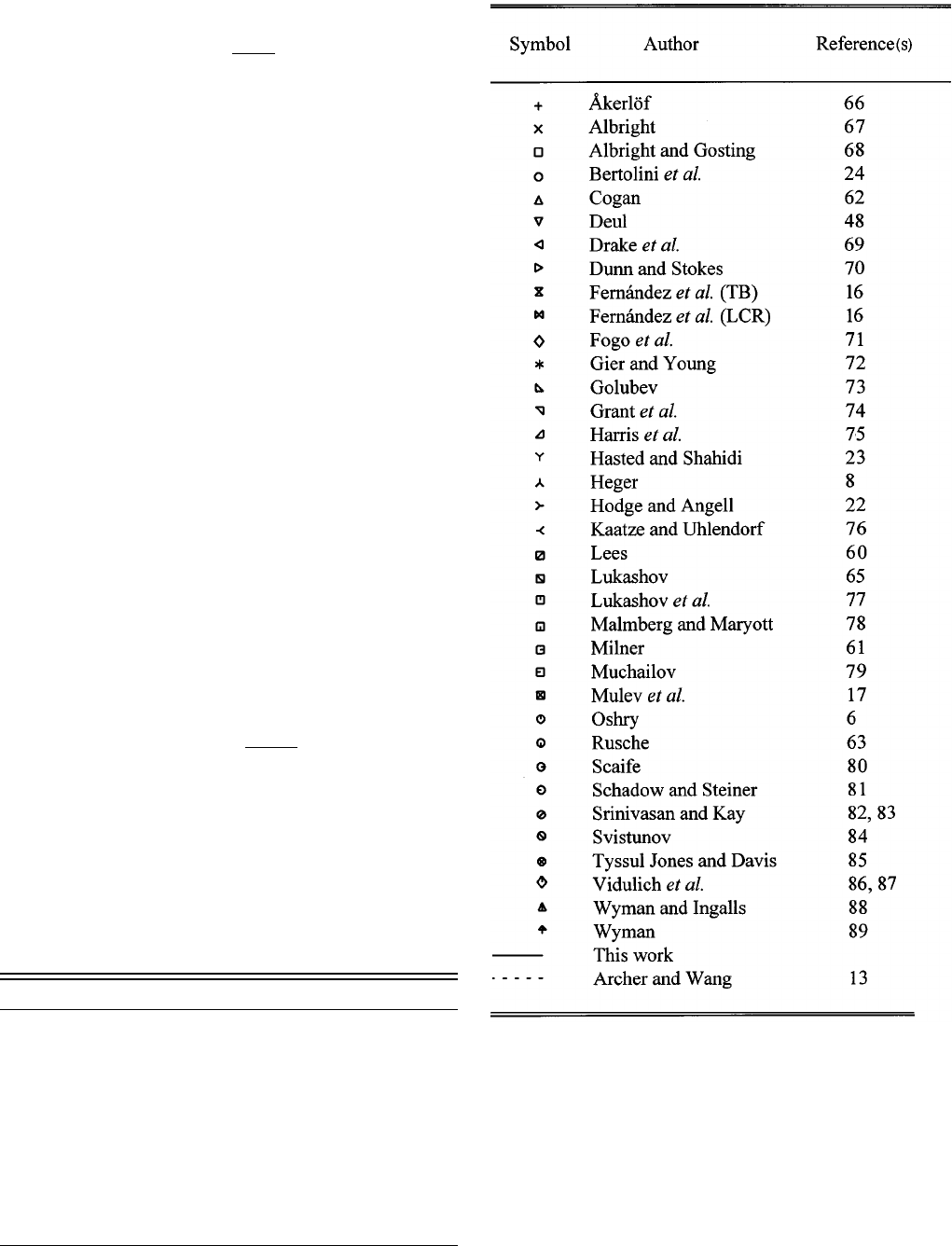
The weight wt for each experimental data point was ob-
tained from:
wt5
1
~
dg
!
2
. ~33!
We based our initial weighting scheme on our data evalu-
ations described in Ref. 3. The uncertainties in the dielectric
constant determined from Ref. 3 are listed in Table 2.
In a preliminary regression analysis with our bank of
terms and the initial weights, we were unable to obtain a
satisfactory equation that represented the dielectric constant
over the entire surface. We therefore adjusted, numerous
times, the bank of terms and found no significant improve-
ment in the equation. Finally, we added additional weights to
key data sets until we obtained an accurate representation of
all dielectric constant data. The data sets, values of g, and
final weights used in the regression analysis and normalized
to sum to unity, are listed in Table 4.
Table 4 shows that while the experimental static dielectric
constant varies between 1 and 110, the corresponding values
of g lie between 1 and 4 in the available temperature and
pressure range. Because of its limited range, g is a more
favorable dependent variable for regression analysis.
5. Results
5.1. Results of the Regression Analysis
The terms selected to represent g were
g5 11
(
k51
11
N
k
~
r
/
r
c
!
i
k
~
T
c
/T
!
j
k
1 N
12
~
r
/
r
c
!
S
T
228 K
2 1
D
2 q
. ~34!
The values of N
k
, i
k
, j
k
, and q are given in Table 5. Each
term entered with a high degree of significance ~.0.9995!
and no further significant terms remained unselected at the
conclusion of the analysis.
5.2. Deviation Plots
The dielectric constant data from virtually the entire data
base
3
are shown in Figs. 5–11 along with the correlation of
Archer and Wang, as deviations from our formulation. The
symbols used are explained in Table 6. In each figure, the
experimental data span small regions of pressure and tem-
perature; the temperature or pressure at which the correlation
TABLE 5. Coefficients N
k
and exponents i
k
, j
k
, and q of Eq. ~34! for the
g-factor.
kN
k
i
k
j
k
1 0.978 224 486 826 1 0.25
2 20.957 771 379 375 1 1
3 0.237 511 794 148 1 2.5
4 0.714 692 244 396 2 1.5
5 20.298 217 036 956 3 1.5
6 20.108 863 472 196 3 2.5
7 0.949 327 488 264• 10
2 1
42
8 20.980 469 816 509• 10
2 2
52
9 0.165 167 634 970• 10
2 4
65
10 0.937 359 795 772• 10
2 4
7 0.5
11 20.123 179 218 720•10
2 9
10 10
12 0.196 096 504 426• 10
2 2
q51.2
T
ABLE 6. Dielectric constant data sources corresponding to the symbols in
the deviation plots.
11401140 FERNANDEZ
ET AL.
J. Phys. Chem. Ref. Data, Vol. 26, No. 4, 1997
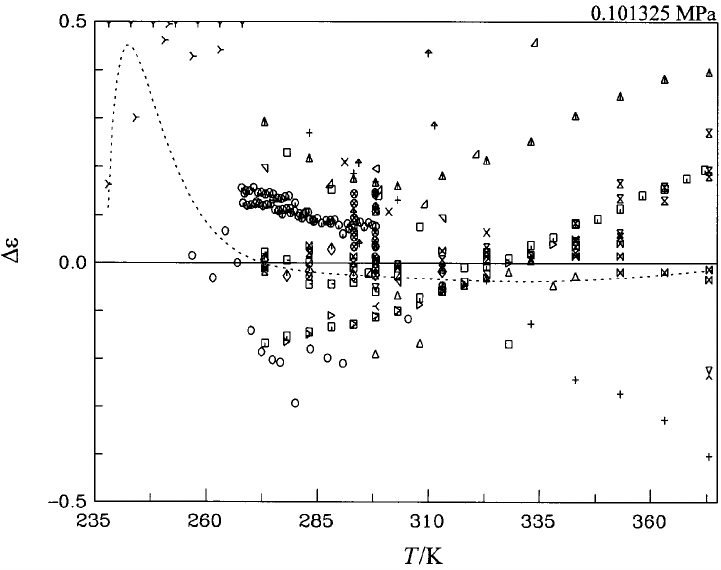
is calculated is indicated in parentheses. Only the data of
Scaife et al.
80
and of Schadow and Steiner
81
were omitted
because they were out of range.
The dielectric constant data at ambient pressure, including
those in the supercooled region, are shown in Fig. 5 as de-
viations from Eqs. ~21! and ~34! plotted against temperature.
For the supercooled state, the data of Hodge and Angell
22
differ from 0.15 to 0.5 from our formulation. This difference
is of similar magnitude as the discrepancy between the
Hodge and Angell data and those of Bertolini et al.
24
at
260 K. The latter measurements and those of Rusche span
both the low temperature liquid and supercooled state, al-
though the minimum temperature reached is well above that
of Hodge and Angell. The Bertolini data lie within 60.1 of
Eqs. ~21! and ~34! in the supercooled region but depart from
the correlation at the higher temperatures, to lie at worst 0.3
below our equation at 283 K. The data of Rusche shows an
opposite trend, converging from an offset of 10.2 at 265 K
to less than 10.1 at about 300 K.
Above 273 K and below 340 K the results of Ferna
´
ndez
et al.,
16
Milner,
61
Cogan,
62
Srinivasan and Kay,
82,83
Lees,
60
and Vidulich et al.
86,87
differ by less than 0.05 from Eqs.
~21! and ~34!, while the data of Malmberg and Maryott
78
and
those of Dunn and Stokes
70
depart systematically below
340 K, to 20.2 below Eqs. ~21! and ~34! at 273.15 K. At
temperatures above 340 K the LCR meter data of Ferna
´
ndez
et al.
17
lie within 0.05 of Eqs. ~21! and ~34! and follow the
trend indicated by the data of Lukhashov,
65
while the
Ferna
´
ndez et al.
17
transformer bridge data follow the trend of
Malmberg and Maryott.
78
At 373 K the latter two data sets
depart from our equation by about 10.2. Above 273 K, the
correlation of Archer and Wang is consistent with ours and
passes through the LCR meter results of Ferna
´
ndez et al.
This agreement implies that the data of Malmberg and Mary-
ott are inconsistent with the other data sets in that range.
The data in liquid water up to 570 K and high pressures
are compared with the formulation in Figs. 6–8. Here com-
parisons are made at narrow temperature intervals around the
nominal values indicated, and the deviations are plotted as a
function of the amount-of-substance density.
The data of Lees
60
extend to densities of about 70
mol dm
2 3
at temperatures between 273 K and 320 K and
therefore anchor the high-density end of the formulation.
They are shown in Figs. 6 and 7. The departures lie within
60.1 of Eqs. ~21! and ~34!, exceeding Lees’s estimated un-
certainty in the measurements ~0.01! but reflecting the actual
scatter of the data. At temperatures between 370 K and
520 K, shown in Fig. 8, the data of Heger
8,12
and Deul
48,49
are inconsistent. At 370 K these two data sets differ by up to
0.5 and they grow further apart at higher temperatures.
The near- and supercritical data are compared in Figs. 9
and 10. The largest difference between the Heger and Deul
data is at 673 K, up to one unit in
e
. At this temperature,
systematic differences from the formulation are of the order
of 60.5. Notwithstanding strenuous effort on our part, the
formulation could not be forced to follow the curvature dis-
played by the Heger data at the high densities. At the highest
temperatures, up to 873 K, the available data are within 60.5
FIG. 5. Deviations D
e
5
e
2
e
~calc.! of dielectric constant
e
data from Eqs. ~21! and ~34!~and coefficients listed in Table 5! for water at a pressure of 0.101325
MPa and temperatures in the range 235–373 K. Symbols: Table 6.
11411141A FORMULATION FOR THE STATIC PERMITTIVITY OF WATER AND STEAM
J. Phys. Chem. Ref. Data, Vol. 26, No. 4, 1997
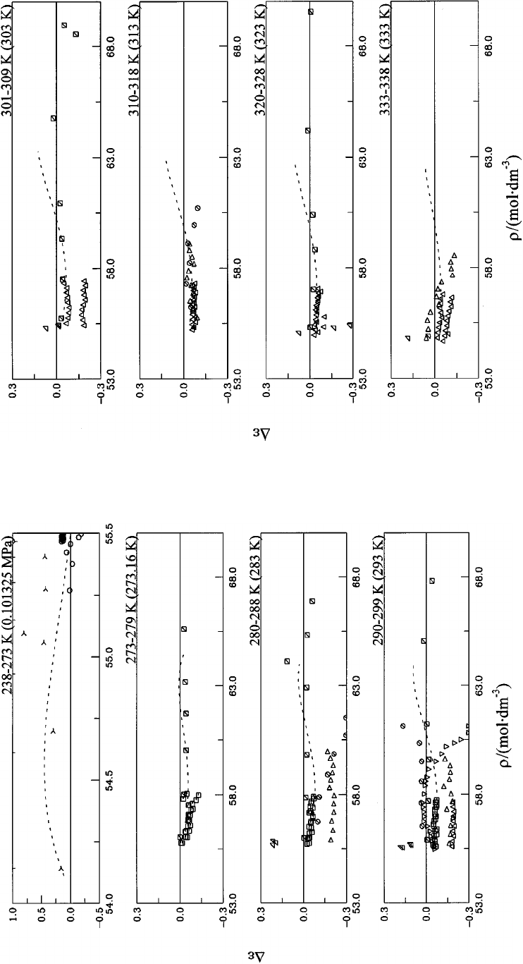
FIG. 6. Deviations D
e
5
e
2
e
~calc.! of dielectric constant
e
data from Eqs. ~21! and ~34!~with
coefficients listed in Table 5! for water at temperatures between 238 K and 299 K. Symbols:
Table 6.
FIG. 7. Deviations D
e
5
e
2
e
~calc.! of dielectric constant
e
data from Eqs. ~21! and ~34!~with
coefficients listed in Table 5! for water at temperatures between 301 K and 338 K. Symbols:
Table 6.
11421142 FERNANDEZ
ET AL.
J. Phys. Chem. Ref. Data, Vol. 26, No. 4, 1997
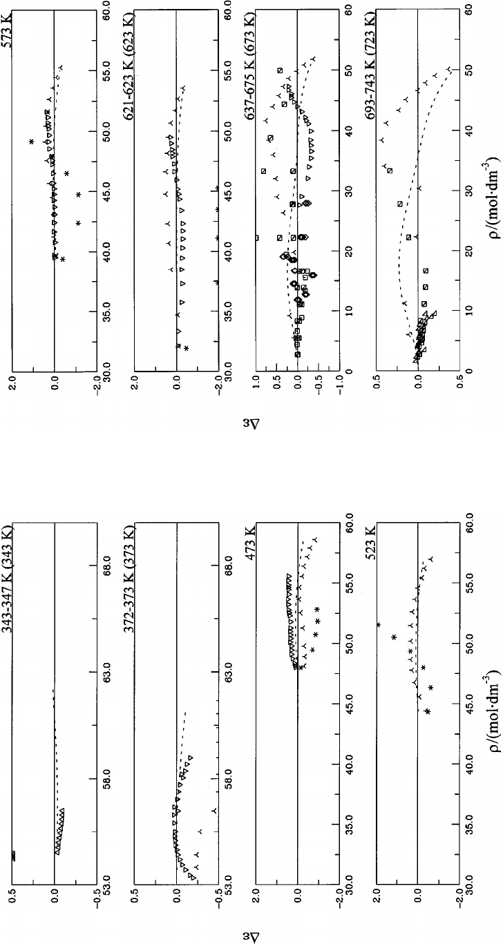
FIG. 8. Deviations D
e
5
e
2
e
~calc.! of dielectric constant
e
data from Eqs. ~21! and ~34!~with
coefficients listed in Table 5! for water at temperatures between 343 K and 523 K. Symbols:
Table 6.
FIG. 9. Deviations D
e
5
e
2
e
~calc.! of dielectric constant
e
data from Eqs. ~21! and ~34!~with
coefficients listed in Table 5! for water at temperatures between 573 K and 743 K. Symbols:
Table 6.
11431143A FORMULATION FOR THE STATIC PERMITTIVITY OF WATER AND STEAM
J. Phys. Chem. Ref. Data, Vol. 26, No. 4, 1997
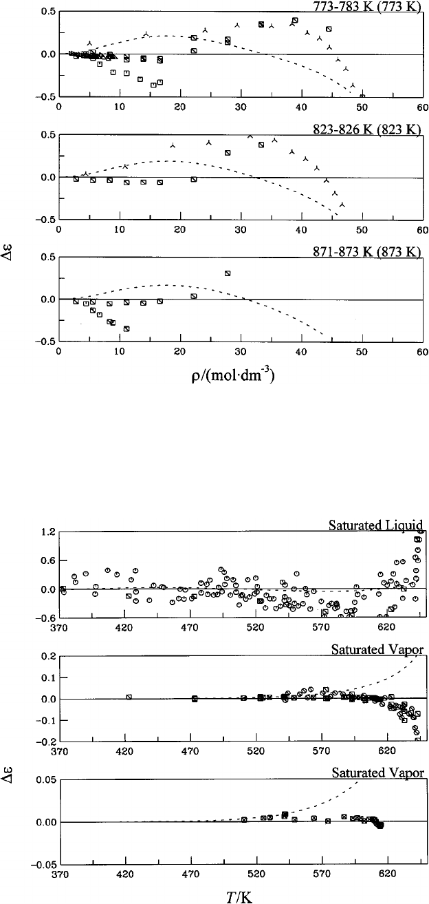
FIG. 10. Deviations D
e
5
e
2
e
~calc.! of dielectric constant
e
data from Eqs. ~21! and ~34!~with coefficients listed in Table 5! for water at temperatures
between 773 K and 873 K. Symbols: Table 6.
FIG. 11. Deviations D
e
5
e
2
e
~calc.! of dielectric constant
e
data from Eqs. ~21! and ~34!~with coefficients listed in Table 5! for saturated liquid water and
steam. Symbols: Table 6.
11441144 FERNANDEZ
ET AL.
J. Phys. Chem. Ref. Data, Vol. 26, No. 4, 1997

from the formulation. In this range, the actual dielectric con-
stant values are of the order of 10 only, so this uncertainty is
substantial.
The saturated liquid and vapor data are shown in Fig. 11.
The saturated liquid data of Lukashov,
65
which were in-
cluded in our regression, and those of Oshry,
6
which were
not, show, albeit small, systematic departures from Eqs. ~21!
and ~34!. These departures increase within the last 25 K from
the critical point, with values up to 1.2 for the liquid, and
down to 20.2 for the vapor, roughly twice the scatter of the
data. The most recent data in the saturated vapor by
Mulev,
3,17
which reach up to 614 K, are in excellent agree-
ment with Eqs. ~21! and ~34!, while the values reported by
Lukashov,
65
Svistunov et al.,
84
and Muchailov
79
depart from
it increasingly as the temperature approaches the critical, and
end up about 0.2 below our formulation.
The theoretical predictions of Goldman et al.
50
are com-
pared with the present formulation in Table 1. In the range of
the data, the theoretical predictions and the formulation dif-
fer by less than one unit in
e
, but the correlation develops
positive departures from the theoretical predictions at the
higher temperatures. For a detailed comparison of SPC/E
computer simulation data with our formulation, see Ref. 59.
The differences between the values obtained from Eqs.
~21! and ~34! and from the correlation of Archer and Wang
13
are less than 0.3 under all conditions. At temperatures below
470 K the differences are less than 0.1 except for the super-
cooled liquid. The two formulations show small systematic
differences at the higher temperatures and densities, which
result from the choice ~and availability! of different data sets
as well as different upper density limits. Archer and Wang,
for instance, included the Heger data
8,12
at subcritical tem-
peratures ~Figs. 8 and 9!, which results in the systematic, but
still quite modest departures between the two formulations in
the high-density range where we choose to follow the Deul
data.
48,49
Nevertheless, the agreement is quite exceptional
and indicates that any uncertainties associated with the selec-
tion of functional form are small compared to the systematics
in the experimental values.
5.3. Comparison with Previous Correlations
At a number of state points, we have compared the current
formulation with the previous formulations of Helgeson and
TABLE 7. Comparison of previous formulations with the present one. ~H&K: Ref. 5: B&P: Ref. 10, U&F: Ref.
11, A&W: Ref. 13!.
T/K
~ITS-90! p/MPa H&K B&P U&F A&W This work
238.00 p
0
*
102.69 106.42 106.31
273.15 p
0
*
87.86 87.81 87.90 87.90
273.15 100 91.69 92.04 91.79 91.84
273.15 500 103.65 101.42 104.71 104.59
273.15 1000 114.23 117.73
298.14 p
0
*
78.47 78.38 78.46 78.38 78.41
298.14 50 80.20 80.17 80.36 80.15 80.21
298.14 100 81.78 81.84 82.08 81.83 81.90
298.14 200 84.38 84.87 84.94 85.00 85.02
298.14 500 90.35 92.24 91.16 93.31 93.09
298.14 1000 101.11 104.60
373.12 p
0
*
55.47 55.46 55.51 55.53
373.12 100 58.55 58.61 58.55 58.67 58.67
373.12 500 66.17 66.95 66.57 67.67 67.78
373.12 1000 73.25 76.39
473.11 100 38.27 38.19 38.17 38.33 38.23
573.11 100 25.46 25.36 25.17 25.10 25.07
673.10 10 1.17 1.25 1.24
673.10 50 12.13 11.24 12.16 12.04 11.99
673.10 100 16.27 17.15 16.05 15.80 15.82
673.10 500 24.68 25.51 24.96 24.63 24.95
673.10 1000 28.64 30.50
773.07 10 1.11 1.17 1.17
773.07 50 3.94 3.45 3.65 3.46
773.07 100 9.27 11.83 9.29 9.05 8.96
773.07 500 18.56 19.14 18.73 19.13
773.07 1000 24.25
873.04 10 1.13 1.13
873.04 50 2.21 2.11
873.04 100 5.53 5.06 4.90
873.04 500 15.83 14.53 14.99
873.04 1000 19.79
1272.96 500 6.34 6.66
*
Liquid state at 0.101 325 MPa.
11451145A FORMULATION FOR THE STATIC PERMITTIVITY OF WATER AND STEAM
J. Phys. Chem. Ref. Data, Vol. 26, No. 4, 1997

Kirkham,
5
Bradley and Pitzer,
10
Uematsu and Franck,
11
and
Archer and Wang.
13
We took tabulated values from the pub-
lished formulations. The results are presented in Table 7.
Blank values in Table 7 indicate entries not present in the
relevant published tables. Data in italics indicate extrapo-
lated values.
5.4. Auxiliary Formulations for Saturated States
Although the formulation gives a complete description of
the dielectric constant both for unsaturated and saturated wa-
ter and steam, it seemed useful to develop separate formula-
tions for the dielectric constant as a function of temperature
for the saturated states, thus circumventing the needs of gen-
erating the saturation boundary from the IAPWS-95 formu-
lation, and incorporating the formulation of the g-factor. The
functional form chosen is such that the limiting behavior at
the critical point is close to theoretical expectations: a 1/3
power law in reduced temperature, with an amplitude of the
same absolute value on the vapor and liquid sides. Defining
the variable
u
5
~
12 T/T
c
!
1/3
~35!
the equation we used to describe the dielectric constant of
the saturated liquid is
e
liq
5 5.36058
S
11
(
i51
i58
L
i
u
i
D
, ~36!
while that for the saturated vapor is given by
e
vap
5 114.36058
S
(
i51,2,7,14,24
V
i
u
i
D
. ~37!
The coefficients in these equations were determined by fit-
ting the functional forms to a dense set of saturation values
generated from the full formulation. The coefficients L
i
and
V
i
are listed in Table 8. The auxiliary equations ~36! and ~37!
represent the dielectric constant values generated by the full
formulation for temperatures up to 634 K to within 0.05%.
Between 634 K and 643 K, the representation agrees with
the full formulation to within 0.1%, and between 643 K and
the critical point, to within 0.5%.
5.5. Reliability Estimates in Various Regions
The reliability estimate of the correlation in each region of
the phase diagram is based on the following three consider-
ations: ~1! our judgement of the quality of the selected data,
if any, for the considered region; ~2! how well the correlation
represents these data; and ~3! the assumption that global av-
eraging tends to yield a result with less uncertainty than that
of the individual data sets. The reliability is quantified by
assigning an uncertainty U
e
(
r
,T), for each region in the
phase diagram. This quantification is not rigorous, and does
not follow the procedures recommended to express experi-
mental uncertainties
94
because the statistical information
needed is mostly not available. The reliability estimates pro-
posed should therefore be considered only as a guideline. We
expect that the dielectric constant for each thermodynamic
condition will be, with a probability close to 1, within the
interval
e
corr
6 U
e
, where
e
corr
is the predicted value from the
present correlation.
Table 9 shows our reliability estimates for the present cor-
relation as a function of temperature and density. Undoubt-
edly the best known region is the liquid phase between
273.15 K and 323.14 K, and pressures up to the freezing
curve. See Ref. 3 for an extensive review and intercompari-
son of the data. At 0.101325 MPa, the data of Lees,
60
Vidu-
lich and Kay,
86,87
and Ferna
´
ndez et al.
16
in this temperature
range agree to within 0.04 units of
e
at 273.15 K, and some-
what closer at the higher temperatures. At 100 MPa, the data
of Lees
60
agree with those of Milner
61
and Cogan
62
within
0.03 units of
e
, or 0.04, at the five temperatures measured by
Lees: 273.15 K, 283.14 K, 293.14 K, 303.13 K and 323.13
K. The formulation fits these data sets closely, and the un-
certainty of the formulation in this range was estimated on
the basis of the agreement with these data sets ~Figs. 6 and
7!.
Above 100 MPa, no direct comparison can be made, but it
TABLE 8. Coefficients L
i
and V
i
for Eqs. ~36! and ~37!.
iL
i
V
i
1 2.725 384 249 466 23.350 389 240 1
2 1.090 337 041 668 23.472 776 251 5
3 21.452 598 367 36
4 247.127 595 811 94
5 4.346 002 813 555
6 237.556 188 697 1
7 2417.735 307 739 7 212.061 801 495
8 249.383 400 313 3
14 225.430 358 103
24 248.297 009 442
TABLE 9. Estimated absolute uncertainty of the predicted dielectric constant,
e
pred
, at various state points.
p/MPa T/K
r
/kg m
2 3
, Ref. 20
e
pred
U
e
p
0
*
238 975.06 106.31 1
p
0
*
256 995.25 95.20 0.3
p
0
*
273 999.83 87.96 0.04
585.3 273 1180 107.06 0.05
p
0
*
323 988.10 69.96 0.04
1189 323 1253 97.02 0.04
p
0
*
373 958.46 55.57 0.2
495.8 373 1110 67.73 0.5
3.16 541 510 15.832 0 1.122 0.003
141.68 523 900 32.23 1
14.757 614 94.3 1.77 0.02
22.038 6 647 357 6.17 0.3
19.933 7 673 100 1.75 0.1
407.896 673 900 23.60 0.5
27.099 773 100 1.66 0.2
581.908 773 900 20.16 0.5
124.707 873 450 6.28 0.4
*
Liquid state at 0.101 325 MPa.
11461146 FERNANDEZ
ET AL.
J. Phys. Chem. Ref. Data, Vol. 26, No. 4, 1997

may be expected that the data of Lees retain an excellent
accuracy. The scatter of the Lees data in this range is less
than 0.1 unit of
e
, or 0.1%, see Figs. 6 and 7, and Fig. 6 in
Ref. 17. These data are fitted to within this scatter, which
forms the basis for an uncertainty estimate in this region.
Above 323.14 K, the uncertainty increases steeply. At the
normal boiling point, the scatter of the most reliable data
sources is at least 0.2 units of
e
, or 0.4%. At pressures higher
than 0.101325 MPa, the uncertainty is higher, due in part to
the discrepancy, close to 1% at 200 MPa, of the only two
data sets, those of Heger
8,12
and Deul.
48,49
For a detailed
discussion of the best values at 298.14 K and 373.12 K, at
0.101325 MPa, see Ref. 3.
At temperatures above 473.12 K and below 873 K, the
dielectric constant is predicted with an uncertainty exceeding
1, with the exception of the vapor phase for temperatures
below 615 K. The saturated-steam state has been investi-
gated accurately
3,17
and a reliability of 0.003
e
units ~better
than 0.3%! is expected for the correlation.
The situation in the rest of the high-temperature region is
fairly uniform. At densities above 500 kg m
2 3
~28
mol m
2 3
), up to the experimental limit corresponding to
pressures of 500 MPa, an uncertainty of 0.5 units of
e
, about
1%, can be expected on the basis of the departures of the
data from the correlation ~Figs. 8–10!. The disagreement be-
tween the Heger and Deul data sets at 673 K, however, oc-
casionally exceeds 1
e
unit or 5% ~Fig. 9!. For the lower
densities, the absolute departures are below 0.5
e
units ~Figs.
9 and 10!, but the relative departures may be several percent,
because of the lower values of
e
.
We have refrained from speculating about the uncertainty
in regions above 873 K. Although we have made sure both
e
and g extrapolate reasonably, there are no data to compare
with. We refer to Sec. 8 for further discussion of this range.
The supercooled region can be divided into two parts.
From 256 K to the normal freezing point, accurate data by
Bertolini et al.
24
measured in the bulk phase agree with the
prediction of the correlation within 0.2 units of
e
, even
though these data were not considered in the fit. Below
256 K, only measurements in dilute emulsions have been
obtained
22
with experimental uncertainties exceeding 1%.
5.6. Tabulation of the Dielectric Constant
Values of the dielectric constant have been calculated on a
grid in p-T space. These values are displayed in Table 19
~Appendix!. Outside the range where data exist, the values
are given in italics and should be considered with caution.
We have taken care to ensure that the equation extrapolates
smoothly as function of temperature and density, but nothing
is known about the uncertainty of the extrapolation. Liquid–
vapor and liquid–solid phase boundaries are indicated. The
values in the supercooled liquid are indicated in bold face.
For the near- and supercritical region, the dielectric con-
stant varies steeply with pressure on isotherms, making in-
terpolation awkward. Representation in a density-
temperature grid ~Table 20! leads to easier interpolation.
6. Derivatives of the Dielectric Constant
6.1. Derivatives Calculated from Experimental
Information
The temperature and pressure derivatives of the dielectric
constant have assumed a huge ~and perhaps somewhat
overblown
95
! importance in the formulation of properties of
aqueous electrolytes because of their role in the Debye–
Hu
¨
ckel limiting law and in applications of the Born model. It
was therefore deemed important to compare derivatives ob-
tained from our formulation with ‘‘experimental’’ values and
with those derived from other formulations.
Several different techniques were employed by us to cal-
culate the first and second derivatives of the dielectric con-
stant with respect to temperature and pressure for experimen-
tal data. All experimental data were sorted by author on
isotherms and isobars. Data that were not isothermal or iso-
baric were not used.
It is important to note that derivatives are not experimen-
tally measured, and that what is termed ‘‘experimental value
of the derivative’’ is, in fact, a value depending on the
method used to derive it from the data. The first technique
we used is a Lagrange interpolation using three and five
points. The method tends to magnify the errors in the experi-
mental data since the polynominal is forced to go through all
points. The second technique we used is a polynomial re-
gression of the data using three to nine terms, which tends to
smooth the data. We tested out the two methods by calculat-
ing the first and second temperature derivatives of the dielec-
tric constant at ambient pressure for the recent data of
Ferna
´
ndez et al.
16
As to the Lagrangian interpolation method, an
(n2 1)
th
-degree polynomial is used to fit a curve through
every point of a set of n unevenly spaced data
e
n
~
x
!
5
(
i51
n
L
i
~
x
!
e
~
x
i
!
, ~38!
where L
i
(x) is given by
L
i
~
x
!
5
)
j5 1,jÞi
n
x2 x
j
x
i
2 x
j
~39!
and x represents the pressure for isothermal data, or the ab-
solute temperature for isobaric data. The value of the number
n is the number of data points used in the interpolation. We
have calculated the derivatives at the experimental data
points themselves, although the Lagrangian interpolation can
be used at any point in the interval. For n5 5, we choose two
data points on each side of the current data point, and for
n5 3, one data point on each side. Near the ends of the
interval, the first, respectively last n data points were used.
The first and second derivatives of
e
with repect to x are
readily obtained from algebraic expressions for the deriva-
tives of L(x).
11471147A FORMULATION FOR THE STATIC PERMITTIVITY OF WATER AND STEAM
J. Phys. Chem. Ref. Data, Vol. 26, No. 4, 1997

In the second method, an n
th
-degree polynomial is fitted to
all data in the experimental range of interest as a function of
one independent variable, while another independent vari-
able is kept constant.
The first and second derivatives of the dielectric constant
with respect to temperature for the Ferna
´
ndez
16
LCR data at
11 different temperatures in the range of 273–373.2 K and at
ambient pressure were determined from 3- and 5-point La-
grangian interpolations, and 3–5 term polynomial fits at
273.174 and 373.113 K. The results are shown in Table 10
for the first and in Table 11 for the second temperature de-
rivative.
Tables 10 and 11 indicate that if all interpolation methods
were considered equivalent, at 273 K, which is the lower
edge of the interval, the first derivative has a 3% uncertainty
at 273 K, and the second derivative is simply not reliably
known. As we mentioned, however, Lagrangian and polyno-
mial interpolations are not at all equivalent, the first method
being the easiest to implement by computer, but having a
tendency to exaggerate the scatter in the derivative, the sec-
ond one smoothing the data, but requiring individual judg-
ment. There are, therefore, no exact guidelines as to how to
choose the proper method. In the case of temperature deriva-
tives of the data of Ferna
´
ndez et al., Tables 10 and 11, we
have opted for the low degree and smoothing features of the
3rd-degree polynomial, and have chosen the uncertainty es-
timates associated with it.
16
In all other calculations of ‘‘ex-
perimental derivatives’’ ~see Section 6.3!, we have opted for
Lagrangian 5-point interpolation for the sake of computation.
6.2. Derivatives from the Correlation
The partial derivative of the dielectric constant with re-
spect to pressure at constant temperature is
S
]
e
]
p
D
T
5
S
]
e
]r
D
T
S
]r
]
p
D
T
. ~40!
The partial derivative of the dielectric constant with respect
to temperature at constant pressure is
S
]
e
]
T
D
p
5
S
]
e
]
T
D
r
2
S
]
e
]r
D
T
S
]
p
]
T
D
r
S
]r
]
p
D
T
. ~41!
From Eqs. ~23!, ~24!, and ~26!, the partial derivative of the
dielectric constant with respect to density at constant tem-
perature is
S
]
e
]r
D
T
54B
1
e
424B
1
A
1
15B
1
10.5C
2 0.5
@
2A
1
1 18B
1
1 2AA
1
110
~
A
1
B1 AB
1
!
118BB
1
#
424B
, ~42!
A and B are defined in Eqs. ~23! and ~24!, respectively, and
A
1
5 A/
r
1
~
A/g
!
S
]
g
]r
D
T
,
B
1
5B/
r
, ~43!
C5 91 2A1 18B1 A
2
1 10AB19B
2
.
The partial derivative of the dielectric constant with respect
to temperature at constant density is
S
]
e
]
T
D
r
5
A
2
1 0.5C
2 0.5
A
2
@
21 2A1 10B
#
42 4B
, ~44!
where
A
2
52A/T1
~
A/g
!
S
]
g
]
T
D
r
. ~45!
The first derivatives were therefore calculated analytically
from the formulation in terms of
r
and T variables, after
which they were converted to derivatives in p, T variables by
multiplying by the appropriate derivatives of the equation of
state. The second derivatives were calculated numerically.
Table 12 presents values of the dielectric constant, and the
two first and three second derivatives. The first part of the
table has integer temperature values on ITS-90, and can be
TABLE 10. Values of (
]
e
/
]
T)
p
determined from the results of Ferna
´
ndez
et al. ~Ref. 16! with five methods at p50.101325 MPa and at temperatures
between 273 K and 373.2 K.
Method 273.174 K 373.113 K
3-point Lagrange 20.3935 20.2571
5-point Lagrange 20.3860 20.2555
3-term polynomial 20.3939 20.2525
4-term polynomial 20.4011 20.2606
5-term polynomial 20.4003 20.2615
mean
a
2 0.39
5
2 0.25
5
6 0.01
2
6 0.01
2
a
Mean 6 2
s
, where
s
is the standard deviation.
TABLE 11. Values of (
]
2
e
/
]
T
2
)
p
determined from the results of Ferna
´
ndez
et al. ~Ref. 16! with five methods at p50.101325 MPa and at temperatures
between 273 K and 373.2 K.
Method 273.174 K 373.113 K
3-point Lagrange 0.003209 0.004195
5-point Lagrange 20.001543 0.001910
3-term polynomial 0.001415 0.001415
4-term polynomial 0.001809 0.001003
5-term polynomial 0.001723 0.000917
mean
a
0.001
2
0.002
1
6 0.003
3
6 0.002
9
a
Mean 6 2
s
, where
s
is the standard deviation.
11481148 FERNANDEZ
ET AL.
J. Phys. Chem. Ref. Data, Vol. 26, No. 4, 1997

used for code checking and other purposes. In the second
part of the table, the temperature entries, all on the ITS-90
scale, have been chosen to correspond with integer Centi-
grade values on the IPTS-68 scale. This part of the table
permits easy comparison with correlations performed prior to
the acceptance of the ITS-90 scale.
The values of the first derivatives with respect to pressure
and temperature are displayed in Figs. 12–21 over the whole
range of the present correlation; the predictions of Ref. 13
are also shown. The first derivatives have a strong infinity at
the water critical point, and are therefore somewhat awkward
to plot in the supercritical regime.
6.3. Comparison of Derivatives from Experiment
and from Correlations
‘‘Experimental’’ values of the first derivatives, obtained
by 5-point Lagrangian interpolation ~Sec. 6.1! are displayed
in Figs. 12–16 ~first pressure derivative!, Figs. 17–21 ~first
temperature derivative!. As argued in Sec. 6.1, Lagrangian
interpolation tends to exaggerate the uncertainty of the de-
rivatives. Therefore, we have additionally performed com-
parisons of first and second temperature and pressure deriva-
tives of the dielectric constant at values of the independent
variables such that experimental information is sufficient to
determine experimental derivatives by polynomial interpola-
TABLE 12. Predicted values of the dielectric constant and its first and second derivatives with respect to pressure and temperature, at selected values of
temperature and pressure.
T/K
~ITS-90! p/MPa
r
/mol dm
23
e
(
]
e
/
]
p)
T
/MPa
2 1
(
]
e
/
]
T)
p
/K
2 1
(
]
2
e
/
]
p
2
)
T
/MPa
2 2
(
]
2
e
/
]
T
2
)
p
/K
2 2
(
]
2
e
/
]
p
]
T)/MPa
2 1
K
2 1
270 p
0
*
55.482 7 89.182 1 0.042 680 5 20.409 375 2 0.567 453 10
2 4
0.226 553 10
2 2
2 0.284 743 10
2 3
300 p
0
*
55.317 4 77.747 4 0.037 186 0 20.355 908 2 0.571 343 10
2 4
0.157 323 10
2 2
2 0.110 073 10
2 3
300 10.0 55.561 5 78.112 7 0.036 634 3 20.357 011 20.543 893 10
2 4
0.160 843 10
2 2
2 0.112 783 10
2 3
300 100.0 57.572 9 81.215 9 0.032 574 8 20.367 852 20.374 923 10
2 4
0.190 413 10
2 2
2 0.124 923 10
2 3
300 1000.0 68.692 7 103.696 0.021 287 2 20.481 815 2 0.503 413 10
2 5
0.357 603 10
2 2
2 0.121 203 10
2 3
350 p
0
*
54.050 2 61.788 9 0.034 827 3 20.284 834 2 0.777 693 10
2 4
0.128 053 10
2 2
2 0.248 203 10
2 5
350 10.0 54.292 2 62.129 9 0.034 083 4 20.284 884 20.726 393 10
2 4
0.129 333 10
2 2
2 0.755 563 10
2 5
350 100.0 56.262 0 64.951 0 0.029 038 3 20.286 956 20.434 403 10
2 4
0.139 093 10
2 2
2 0.339 723 10
2 4
350 1000.0 67.295 1 83.608 4 0.016 893 2 20.334 865 20.444 153 10
2 5
0.215 763 10
2 2
2 0.574 913 10
2 4
400 10.0 52.312 2 49.385 0 0.035 083 9 20.227 249 20.106 473 10
2 3
0.101 243 10
2 2
0.461 033 10
2 4
400 100.0 54.499 5 52.200 9 0.028 247 8 20.225 663 20.546 193 10
2 4
0.107 523 10
2 2
2 0.152 323 10
2 5
400 1000.0 65.942 2 69.124 9 0.014 787 2 20.251 380 20.423 343 10
2 5
0.131 473 10
2 2
2 0.320 723 10
2 4
450 10.0 49.744 7 39.171 6 0.038 933 6 20.183 607 20.177 953 10
2 3
0.734 303 10
2 3
0.113 973 10
2 3
450 100.0 52.372 9 42.149 5 0.028 741 0 20.178 549 20.731 293 10
2 4
0.816 623 10
2 3
0.211 913 10
2 4
450 1000.0 64.598 3 58.020 0 0.013 401 1 20.195 865 20.402 223 10
2 5
0.943 873 10
2 3
2 0.246 403 10
2 4
500 10.0 46.517 5 30.794 1 0.047 663 0 20.153 818 20.362 983 10
2 3
0.453 623 10
2 3
0.256 633 10
2 3
500 100.0 49.914 0 34.149 0 0.030 425 4 20.143 247 20.104 113 10
2 3
0.603 423 10
2 3
0.472 113 10
2 4
500 1000.0 63.253 0 49.301 7 0.012 264 8 20.154 787 20.390 983 10
2 5
0.712 693 10
2 3
2 0.210 353 10
2 4
550 10.0 42.287 5 23.530 8 0.069 541 0 20.139 993 20.109 163 10
2 2
0.487 653 10
2 4
0.733 663 10
2 3
550 100.0 47.114 6 27.667 2 0.033 596 6 20.117 403 20.157 343 10
2 3
0.438 233 10
2 3
0.812 803 10
2 4
550 1000.0 61.909 0 42.377 5 0.011 287 8 20.123 594 20.390 183 10
2 5
0.543 043 10
2 3
2 0.180 893 10
2 4
600 100.0 43.934 6 22.290 3 0.038 745 0 20.098 672 4 2 0.251 403 10
2 3
0.318 103 10
2 3
0.126 803 10
2 3
600 1000.0 60.571 5 36.819 5 0.010 451 9 20.099 791 5 2 0.397 003 10
2 5
0.415 103 10
2 3
2 0.153 893 10
2 4
650 100.0 40.310 9 17.717 3 0.046 488 1 20.084 898 7 2 0.419 463 10
2 3
0.239 963 10
2 3
0.184 543 10
2 3
650 1000.0 59.246 1 32.305 8 0.009 7437 7 20.081 552 1 2 0.408 423 10
2 5
0.319 143 10
2 3
2 0.129 953 10
2 4
700 100.0 36.179 0 13.754 4 0.057 134 6 20.073 855 7 2 0.699 433 10
2 3
0.211 783 10
2 3
0.236 223 10
2 3
700 1000.0 57.937 2 28.595 1 0.009 146 26 20.067 471 6 2 0.421 913 10
2 5
0.247 593 10
2 3
2 0.109 693 10
2 4
750 100.0 31.557 5 10.336 0 0.068 683 4 20.062 523 6 2 0.102 203 10
2 2
0.254 473 10
2 3
0.198 463 10
2 3
750 1000.0 56.648 9 25.507 2 0.008 640 69 20.056 489 7 2 0.435 573 10
2 5
0.194 283 10
2 3
2 0.931 413 10
2 5
800 100.0 26.767 6 7.562 25 0.073 445 0 20.047 827 0 20.980 763 10
2 3
0.322 803 10
2 3
2 0.301 963 10
2 4
800 1000.0 55.384 2 22.907 7 0.008 209 19 20.047 821 0 2 0.448 013 10
2 5
0.154 373 10
2 3
2 0.799 813 10
2 5
273.150 p
0
*
55.499 8 87.903 5 0.041 829 7 20.402 570 2 0.550 723 10
2 4
0.206 743 10
2 2
2 0.256 173 10
2 3
273.150 100.0 58.021 8 91.838 0 0.037 176 5 20.426 331 20.401 523 10
2 4
0.261 833 10
2 2
2 0.219 823 10
2 3
298.144 p
0
*
55.344 7 78.410 6 0.037 396 6 20.358 840 2 0.566 063 10
2 4
0.158 703 10
2 2
2 0.116 893 10
2 3
298.144 50.0 56.532 1 80.211 4 0.034 873 6 20.364 953 20.453 773 10
2 4
0.176 683 10
2 2
2 0.126 883 10
2 3
298.144 200.0 59.500 1 85.017 5 0.029 695 0 20.384 517 20.256 723 10
2 4
0.221 953 10
2 2
2 0.130 703 10
2 3
373.124 p
0
*
53.197 5 55.533 3 0.035 099 4 20.256 700 2 0.925 183 10
2 4
0.115 253 10
2 2
0.252 663 10
2 4
373.124 100.0 55.496 2 58.672 7 0.028 474 7 20.256 655 20.479 093 10
2 4
0.123 413 10
2 2
2 0.160 423 10
2 4
473.110 100.0 51.277 4 38.231 7 0.029 358 8 20.160 903 20.854 493 10
2 4
0.712 143 10
2 3
0.324 583 10
2 4
673.102 100.0 38.467 6 15.818 0 0.051 073 6 20.079 613 0 2 0.533 993 10
2 3
0.219 523 10
2 3
0.212 053 10
2 3
773.071 100.0 29.331 4 8.964 72 0.072 338 6 20.056 201 7 20.107 333 10
2 2
0.293 683 10
2 3
0.110 283 10
2 3
*
Liquid state at 0.101 325 MPa.
11491149A FORMULATION FOR THE STATIC PERMITTIVITY OF WATER AND STEAM
J. Phys. Chem. Ref. Data, Vol. 26, No. 4, 1997
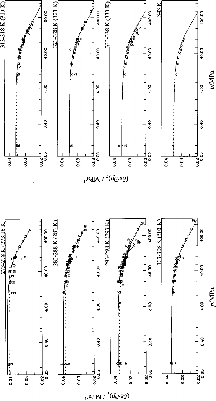
FIG. 12. First derivative of the dielectric constant with respect to pressure at constant temperature
(
]
e
/
]
p)
T
for water at temperatures between 273 K and 308 K. Symbols: Table 6; ‘‘experimen-
tal’’ values: 5-point Lagrangian interpolation. Dashed curve: Ref. 13.
FIG. 13. First derivative of the dielectric constant with respect to pressure at constant temperature
(
]
e
/
]
p)
T
for water at temperatures between 313 K and 343 K. Symbols: Table 6; ‘‘experimen-
tal’’ values: 5-point Lagrangian interpolation. Dashed curve: Ref. 13.
11501150 FERNANDEZ
ET AL.
J. Phys. Chem. Ref. Data, Vol. 26, No. 4, 1997
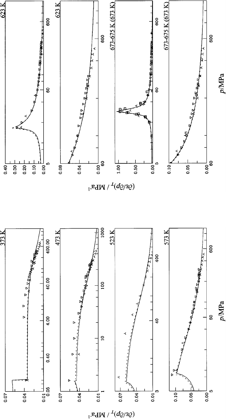
FIG. 14. First derivative of the dielectric constant with respect to pressure at constant temperature
(
]
e
/
]
p)
T
for water at temperatures between 373 K and 573 K. Symbols: Table 6; ‘‘experimen-
tal’’ values: 5-point Lagrangian interpolation. Dashed curve: Ref. 13.
FIG. 15. First derivative of the dielectric constant with respect to pressure at constant temperature
(
]
e
/
]
p)
T
for water at temperatures between 623 K and 675 K. Symbols: Table 6; ‘‘experimen-
tal’’ values: 5-point Lagrangian interpolation. Dashed curve: Ref. 13.
11511151A FORMULATION FOR THE STATIC PERMITTIVITY OF WATER AND STEAM
J. Phys. Chem. Ref. Data, Vol. 26, No. 4, 1997
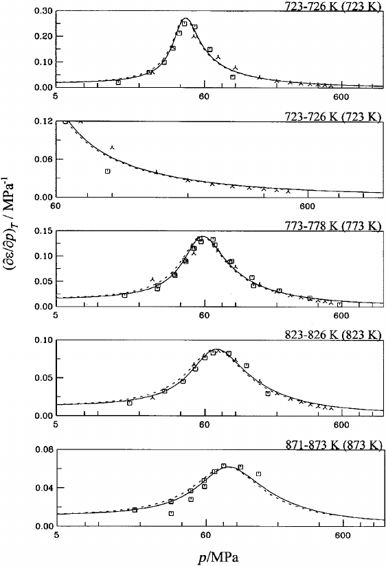
tion. Six isotherms in the range 273–673.1 K have been
selected, and one to three target pressures have been chosen
at each temperature.
Tables 13–16 contain values for first and second pressure
and temperatures derivatives derived from experimental data
by low-degree polynomial fits along isotherms or isobars
~Sec.6.2!; they are listed under the heading ‘‘experiments.’’
In addition, derivative values for the same table entries have
been calculated for the correlations of Helgeson and
Kirkham,
5
Bradley and Pitzer,
10
and Archer and Wang.
13
The last line in the tables contains the values predicted by the
present correlation.
At 273.15 K and 0.1 MPa, the first temperature derivative
values shown in Table 13 agree within 1%, except for the
values derived from Milner’s data. The values obtained by
polynomial fits to the data of Lees,
60
Vidulich et al.,
86,87
and
Ferna
´
ndez et al.
16
agree to the third digit. The value resulting
from the correlation of Bradley and Pitzer
10
is somewhat low
in absolute value, probably because the authors relied on the
data by Dunn and Stokes
70
in this region; these data, and
those by Malmberg and Maryott,
78
depart from those of
Refs. 60, 85, 86, and 16, which were preferred by us. The
value resulting from the Archer and Wang correlation,
20.405 K
2 1
, seems somewhat high in absolute value with
respect to the experimental average ~Milner’s data excluded!
of 20.402 K
2 1
. These authors did not have the new data
16
available when they did their correlation.
At 298.14 K and ambient pressure, uncertainties in the
first temperature derivative are below 1%, with some dete-
rioration at elevated pressures.
At temperatures higher than 373.12 K, first temperature
derivative values obtained from the Heger
8,12
and the
Deul
48,49
data disagree sharply, and so do the differences
between the various correlations. The predictions of the two
most recent correlations, however, agree remarkably well,
notwithstanding vastly different functional forms.
FIG. 16. First derivative of the dielectric constant with respect to pressure at constant temperature (
]
e
/
]
p)
T
for water at temperatures between 723 K and 873
K. Symbols: Table 6; ‘‘experimental’’ values: 5-point Lagrangian interpolation. Dashed curve: Ref. 13.
11521152 FERNANDEZ
ET AL.
J. Phys. Chem. Ref. Data, Vol. 26, No. 4, 1997
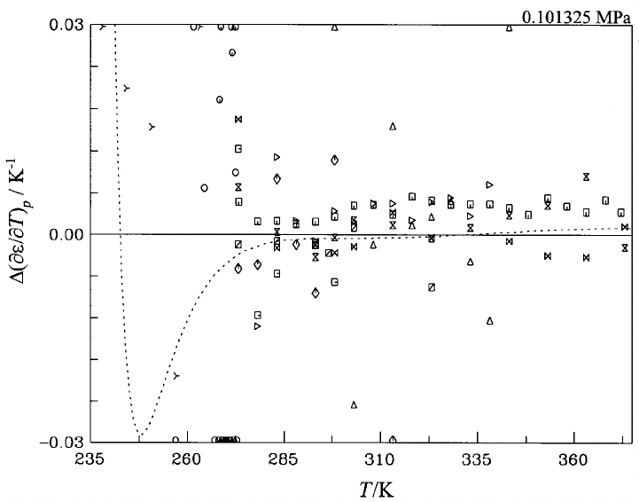
The second temperature derivative at ambient pressure and
up to the boiling point is shown in Table 14. At the normal
freezing point, the spread of experimental derivative values
and predictions from correlations exceeds 10%. The uncer-
tainty in the second temperature derivative in the super-
cooled regime must be at least that large. As the temperature
increases above the freezing point, the uncertainty of the
second temperature derivative falls, and at 298.14 K the
spread of values is well below 10%.
Above 373.12 K, the predictions from the different corre-
lations agree in the order of 10%, much better than the val-
ues calculated from the various data sets. The agreement
between the two most recent formulations, however, is re-
markable.
The values of the first and second pressure derivatives are
shown in Tables 15 and 16, respectively. Especially for the
second derivatives, the experimental values show large scat-
ter.
It is worth noting that the derivative values obtained from
the correlations are generally much better defined than the
values derived from individual experimental data sets. The
various correlations, though of very different algebraic
forms, apparently do comparable jobs of smoothing the data,
even in regions where there are few and not very consistent
data. This is especially striking for the two most recent for-
mulations.
6.4. Reliability of the Derivatives
of the Dielectric Constant
Tables 13–16 permit us to estimate the reliability of the
dielectric constant derivatives, by comparing values obtained
from the four different high-quality correlations. This is, of
course, a somewhat optimistic estimate of uncertainty since
all these formulations, in regions where data are sparse or
inconsistent, might try to fit to a set of unconfirmed data
which could be wrong.
The first temperature derivative ~Table 13! is defined
within 1% up to the boiling point, with a somewhat larger
spread ~1.5%! at 273 K, at the low end of the range. At the
higher temperatures, up to 673 K, the differences mostly re-
main within 10%. The definition of the second temperature
derivative ~Table 14! is, of course, much worse, with a
percent-level definition only in the middle of the range, 298–
373 K. At the 273 K end, the derivative values scatter by
25%.
The first pressure derivative ~Table 15! spreads no more
than 3% up to 473 K. Above that temperature, the spread is
within 10%. The second pressure derivative is poorly defined
almost everywhere.
In general, the differences between the present formulation
and that of Archer and Wang are smaller than the overall
spread between formulations.
A legitimate question is that of the effect of the equation
FIG. 17. Departure from the formulation for the first derivative of the dielectric constant with respect to temperature at constant pressure (
]
e
/
]
T)
p
for water
at 0.101325 MPa in the range of 235–373 K. Symbols: Table 6; ‘‘experimental’’ values: 5-point Lagrangian interpolation. Dashed curve: Ref. 13.
11531153A FORMULATION FOR THE STATIC PERMITTIVITY OF WATER AND STEAM
J. Phys. Chem. Ref. Data, Vol. 26, No. 4, 1997
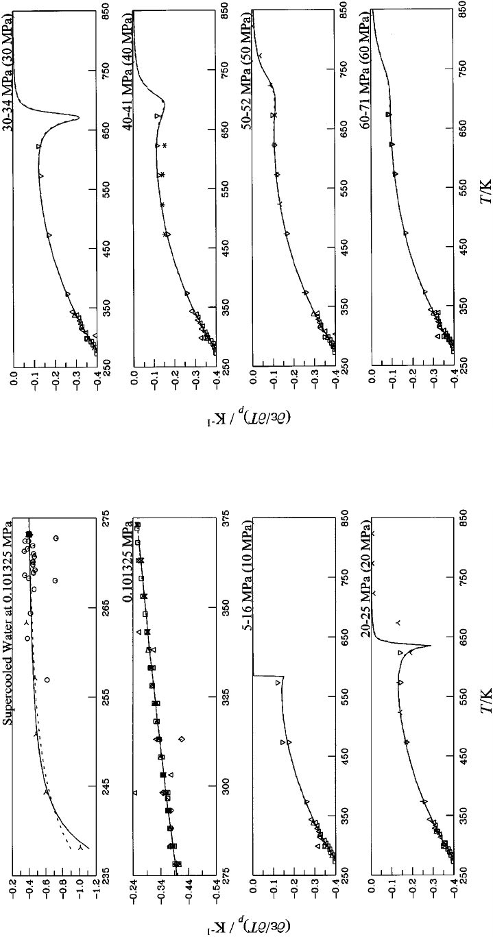
FIG. 18. First derivative of the dielectric constant with respect to temperature at constant pressure
(
]
e
/
]
T)
p
for water at pressures between 0.1 MPa and 25 MPa. Symbols: Table 6; ‘‘experimen-
tal’’ values: 5-point Lagrangian interpolation. Dashed curve: Ref. 13.
FIG. 19. First derivative of the dielectric constant with respect to temperature at constant pressure
(
]
e
/
]
T)
p
for water at pressures between 30 MPa and 71 MPa. Symbols: Table 6; ‘‘experimen-
tal’’ values: 5-point Lagrangian interpolation. Dashed curve: Ref. 13.
11541154 FERNANDEZ
ET AL.
J. Phys. Chem. Ref. Data, Vol. 26, No. 4, 1997
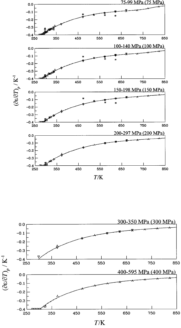
FIG. 20. First derivative of the dielectric constant with respect to temperature at constant pressure (
]
e
/
]
T)
p
for water at pressures between 75 MPa and 297
MPa. Symbols: Table 6; ‘‘experimental’’ values: 5-point Lagrangian interpolation. Dashed curve: Ref. 13.
FIG. 21. First derivative of the dielectric constant with respect to temperature at constant pressure (
]
e
/
]
T)
p
for water at pressures between 300 MPa and
595 MPa. Symbols: Table 6; ‘‘experimental’’ values: 5-point Lagrangian interpolation. Dashed curve: Ref. 13.
11551155A FORMULATION FOR THE STATIC PERMITTIVITY OF WATER AND STEAM
J. Phys. Chem. Ref. Data, Vol. 26, No. 4, 1997

TABLE 14. Second temperature derivative of the dielectric constant at constant pressure.
10
5
(
]
2
e
/
]
T
2
)
p
/K
2 2
T/K→
273.15 298.14 373.12 473.11 573.11 673.10
p/MPa→ p
0
*
100 p
0
*
100 200 p
0
*
100 100 100 100
Experiments
Wyman
89
Lees
60
196 170 196 219
Milner
61
250 202 250 180
Vidulich et al.
87
166
Heger
8
143 74 33 19
Deul
48
215 129 63 36 50
Ferna
´
ndez et al.
16
185 165 109
Correlations
Helgeson & Kirkham
5
130 117 128 73 34 19
Bradley & Pitzer
10
154 209 155 183 208 114 124 74 45
Archer & Wang
13
240 351 159 194 218 116 125 69 38 24
This work 207 262 159 193 222 115 123 711 38 22
*
Liquid state at 0.101 325 MPa.
TABLE 15. First pressure derivative of the dielectric constant at constant temperature.
10
4
(
]
e
/
]
p)
T
/MPa
2 1
T/K→
273.15 298.14 373.12 473.11 673.10 773.07
p/MPa→ p
0
*
100 p
0
*
50 200 p
0
*
100 100 100 100
Experiments
Lees
60
406 371
Milner
61
383 370 347
Cogan
62
369 347
Heger
8
327 273 315 487 640
Srinivasan
82
372 349 301
Lukashov
65
787
Deul
48
381 358 278 378 291 300 528
Correlations
Helgeson & Kirkham
5
366 329 262 352 281 299 568 746
Bradley & Pitzer
10
407 361 371 345 286 353 283 301
Archer & Wang
13
407 371 365 344 305 357 284 294 503 695
This work 418 372 374 349 297 351 285 294 511 723
*
Liquid state at 0.101 325 MPa.
TABLE 13. First temperature derivative of the dielectric constant at constant pressure.
2 10
3
(
]
e
/
]
T)
p
/K
2 1
T/K→
273.15 298.14 373.12 473.11 573.11 673.10
p/MPa→ p
0
*
100 p
0
*
100 200 p
0
*
100 100 100 100
Experiments
Wyman
89
360 257
Lees
60
402 422 360 373 386
Milner
61
411 428 358 366 382
Vidulich et al.
87
402 360
Heger
8
262 156 104 81
Deul
48
377 385 253 160 114 75
Ferna
´
ndez et al.
16
402 359 258
Correlations
Helgeson & Kirkham
5
357 368 371 258 258 157 104 81
Bradley & Pitzer
10
398 419 359 370 382 257 257 160 101 65
Archer & Wang
13
405 432 359 370 384 256 255 161 109 79
This work 403 426 359 371 385 257 257 161 108 80
*
Liquid state at 0.101 325 MPa.
11561156 FERNANDEZ
ET AL.
J. Phys. Chem. Ref. Data, Vol. 26, No. 4, 1997

TABLE 16. Second pressure derivative of the dielectric constant at constant temperature.
2 10
6
(
]
2
e
/
]
p
2
)
T
/MPa
2 2
T/K→
273.15 298.14 373.12 473.11 673.10 773.07
p/MPa→ p
0
*
100 p
0
*
50 200 p
0
*
100 100 100 100
Experiments
Lees
60
41 35
Milner
61
30 23 66 51
Cogan
62
68 43
Heger
8
66 54 90 343 483
Srinivasan
82
63 52 11
Lukashov
65
860
Deul
48
59 57 50 117 78 103 418
Correlations
Helgeson & Kirkham
5
104 54 124 45 109 586 971
Bradley & Pitzer
10
51 40 55 48 33 87 56 104
Archer & Wang
13
39 31 46 35 21 106 51 95 529 1047
This work 55 40 57 45 26 93 48 85 534 1073
*
Liquid state at 0.101 325 MPa.
TABLE 17. Predicted values of the Debye–Hu
¨
ckel coefficients at selected values of temperature and pressure.
Values in italics are outside the range of experimental data.
T/K
~ITS-90!
p/MPa A
f
(kg mol
21
!
1/2
A
V
~cm
3
kg
1/2
mol
23/2
)
A
H
/RT
(kg mol
21
!
1/2
A
K
~cm
3
kg
1/2
mol
23/2
MPa
21
)
A
C
/R
(kg mol
21
!
1/2
270 p
0
*
0.374 75 1.537 5 0.564 28 20.002 473 6 1.761 1
300 p
0
*
0.392 51 1.927 5 0.814 48 20.004 340 9 3.901 4
300 10.0 0.390 62 1.885 7 0.803 15 20.004 110 1 3.813 9
300 100.0 0.375 05 1.585 4 0.726 66 20.002 720 0 3.152 4
300 1000.0 0.283 96 0.702 18 0.600 01 20.000 435 37 1.257 5
350 p
0
*
0.434 57 3.118 3 1.409 8 20.010 397 6.132 7
350 10.0 0.431 96 3.019 1 1.382 1 20.009 657 1 5.956 4
350 100.0 0.411 39 2.362 5 1.189 1 20.005 527 3 4.783 9
350 1000.0 0.308 07 0.864 45 0.655 07
2
0.000 555 01 1.303 0
400 10.0 0.489 72 5.223 4 2.129 1 20.023 563 9.021 8
400 100.0 0.459 96 3.752 2 1.748 5 20.011 390 6.611 4
400 1000.0 0.332 02 1.131 9 0.797 37
2
0.000 793 40 2.205 0
450 10.0 0.566 54 9.671 8 3.182 3 20.064 731 14.964
450 100.0 0.520 81 6.113 2 2.421 2 20.024 311 9.184 7
450 1000.0 0.358 14 1.492 3 0.981 33
2
0.001 130 0 2.636 7
500 10.0 0.671 09 20.023 4.981 1 20.219 66 29.970
500 100.0 0.595 28 10.230 3.293 4 20.054 486 13.512
500 1000.0 0.386 30 1.933 1 1.156 3
2
0.001 579 7 2.797 3
550 10.0 0.830 30 52.399 9.159 3 21.160 8 86.227
550 100.0 0.687 41 17.800 4.544 7 20.130 08 21.426
550 1000.0 0.415 68 2.452 0 1.308 4
2
0.002 167 2 2.853 6
600 100.0 0.805 62 32.686 6.512 8 20.335 65 36.568
600 1000.0 0.445 57 3.052 6 1.438 8
2
0.002 922 2 2.895 5
650 100.0 0.965 77 64.214 9.843 7 20.946 29 66.458
650 1000.0 0.475 52 3.742 1 1.553 4
2
0.003 878 5 2.967 7
700 100.0 1.196 9 135.69 15.739 22.883 6 124.09
700 1000.0 0.505 27 4.529 3 1.658 4
2
0.005 071 9 3.088 0
750 100.0 1.547 2 299.47 25.776 28.726 7 209.94
750 1000.0 0.534 74 5.424 4 1.759 1
2
0.006 538 9 3.257 9
800 100.0 2.066 9 616.62 38.835 220.833 239.33
800 1000.0 0.563 92 6.437 4 1.859 2
2
0.008 315 3 3.469 5
273.150 p
0
*
0.376 41 1.570 8 0.580 68 20.002 615 4 2.191 9
273.150 100.0 0.360 40 1.352 3 0.538 60 20.001 884 7 1.924 9
298.144 p
0
*
0.391 26 1.897 8 0.795 51 20.004 196 5 3.820 3
298.144 50.0 0.382 19 1.713 2 0.747 24 20.003 274 5 3.423 9
298.144 200.0 0.359 32 1.346 3 0.664 57 20.001 815 0 2.566 8
373.124 p
0
*
0.459 69 4.010 1 1.741 5 20.015 715 7.439 5
373.124 100.0 0.432 34 2.914 0 1.436 3 20.007 695 9 5.581 2
473.110 100.0 0.553 37 7.724 9 2.791 3 20.035 059 10.882
673.102 100.0 1.061 3 89.955 12.151 21.572 3 88.779
773.071 100.0 1.764 7 425.76 31.748 213.633 238.49
*
Liquid state at 0.101 325 MPa.
11571157A FORMULATION FOR THE STATIC PERMITTIVITY OF WATER AND STEAM
J. Phys. Chem. Ref. Data, Vol. 26, No. 4, 1997
of state in those formulations that use a g-factor as a function
of density. It is our opinion that the variations in the equa-
tions of state used will have a rather minor effect, because
any uncertainties introduced into the density when calculated
from measured pressures will be compensated for by the fit
of the g-factor. In other words, the fit is to the dielectric
constant data, and if they are fitted well, it does not matter if
the equation of state was not perfect. The quality of the equa-
tion of state, however, definitely affects the reliability of the
Debye–Hu
¨
ckel coefficients.
7. Debye–Hu
¨
ckel Coefficients
7.1. Definition and Values
The Debye–Hu
¨
ckel limiting law for electrolyte solutions
was originally formulated in terms of a Helmholtz free en-
ergy framework,
1
and describes the concentration depen-
dence of thermodynamic properties due to the presence of
ionic charges in the limit of infinite dilution. In applications
to aqueous electrolyte solutions, the limiting-law term is in-
corporated in the Gibbs free energy. This is allowed as long
as the fluid has low compressibility, see, however, Ref. 95.
The limiting law defines an initial slope for the concentration
dependence of each of the excess thermodynamic properties:
Gibbs free energies of solvent and solute, and apparent molar
volume, enthalpy, heat capacity and compressibility of the
solute. When formulated in terms of the excess Gibbs free
energy, it is based on the pure-solvent and infinite-dilution
solute standard states and on the molality scale for
concentration.
96–99
The coefficient A
g
multiplying the
Debye–Hu
¨
ckel composition dependence for the logarithm of
the activity coefficient of the solute has the following
form:
96,97
A
g
5
~
2
p
N
A
r
M
w
!
1/2
@
e
2
/
~
4
p
ee
0
kT
!
#
3/2
. ~46!
From the Debye–Hu
¨
ckel coefficient for the limiting slope of
the activity, Debye–Hu
¨
ckel coefficients for the limiting
slopes of other thermodynamic properties are derived by dif-
ferentiation, as follows. For that of the osmotic coefficient
97
A
f
5 A
g
/3. ~47!
For that of the apparent molar volume
98
A
V
524RT
~
]
A
f
/
]
p
!
T
. ~48!
For that of the apparent molar compressibility
10
A
K
5
~
]
A
V
/
]
p
!
T
. ~49!
For that of the apparent molar enthalpy
10,97
A
H
/RT54T
~
]
A
f
/
]
T
!
p
. ~50!
For that of the apparent molar heat capacity
97
A
C
5
~
]
A
H
/
]
T
!
p
. ~51!
Here e is the charge of the electron, R is the universal gas
constant,
r
is the molar density, and M
w
the molar mass of
water, see Table 3.
The expressions used to calculate the Debye–Hu
¨
ckel co-
efficients for the apparent molar volume and enthalpy are,
respectively,
A
V
5 2A
f
RT
@
3
~
]
e
/
]
p
!
T
/
e
2
~
]r
/
]
p
!
T
/
r
#
, ~52!
A
H
526A
f
RT
@
11T
~
]
e
/
]
T
!
p
/
e
2T
~
]r
/
]
T
!
p
/3
r
#
. ~53!
The higher-order derivatives were calculated numerically.
The units of A
f
, A
H
/RT, and A
C
/R are ~kg mol
2 1
)
1/2
,
that of A
V
is cm
3
kg
1/2
mol
2 3/2
and that of A
K
,
cm
3
kg
1/2
mol
2 3/2
MPa
2 1
.
The expressions for the Debye–Hu
¨
ckel coefficients con-
tain, in addition to the first and second pressure and tempera-
ture derivatives of the dielectric constant, also the first and
second derivatives of the equation of state.
Table 17 displays the values of the Debye–Hu
¨
ckel coeffi-
cients derived from the present formulation for the same
choices of temperature and density entries as in Table 12. As
in Table 12, the bottom part of Table 17 is produced at
ITS-90 temperatures that correspond with integer values of
the IPTS-68 Centigrade scale. It can be used for comparison
with predictions made on that scale by earlier workers. The
top part of the table is at integer temperatures on the ITS-90
Kelvin scale. An excessive number of decimals is given, sev-
eral more than the reliability of these values warrants; the
purpose is to permit code checking.
7.2. Reliability
As a first measure of the reliability of the Debye–Hu
¨
ckel
coefficients, the uncertainty of the derivatives of the dielec-
tric constant, as determined in Section 6, can be used as a
guide. This implies a few percent or less uncertainty in the
first derivatives, 10% or more in the second temperature de-
rivative except for the range of ambient-pressure liquid water
~1%–1.5%!, 10% or less in the first pressure derivative, and
an undefined second pressure derivative.
In addition, however, the derivatives of the equation of
state itself explicitly enter into the picture, see, for instance,
Eqs. ~52! and ~53!. It is natural to assume that the equation of
state, being based on a very large body of excellent thermo-
dynamic data, does not contribute to the uncertainty of the
Debye–Hu
¨
ckel coefficients. This is, however, not true. As an
example, in Fig. 22, the second temperature derivative, as
calculated from different high quality equations of state,
those of Haar et al.,
100
Saul and Wagner,
101
Hill,
14
and Wag-
ner and Pruss,
19,20
is displayed as a function of the pressure
along isotherms at 253 K, 273 K, and 298 K. It is obvious
that at 253 K and 273 K, this derivative is not defined at the
higher pressures. Also, second derivatives of some of these
accurate equations of state display unphysical oscillations in
the subcooled liquid.
An exhaustive investigation of the behavior of the deriva-
tives of the equation of state is beyond the scope of this
paper, and will be the topic of future research. A cursory
check in other regions of phase space, including the super-
11581158 FERNANDEZ
ET AL.
J. Phys. Chem. Ref. Data, Vol. 26, No. 4, 1997
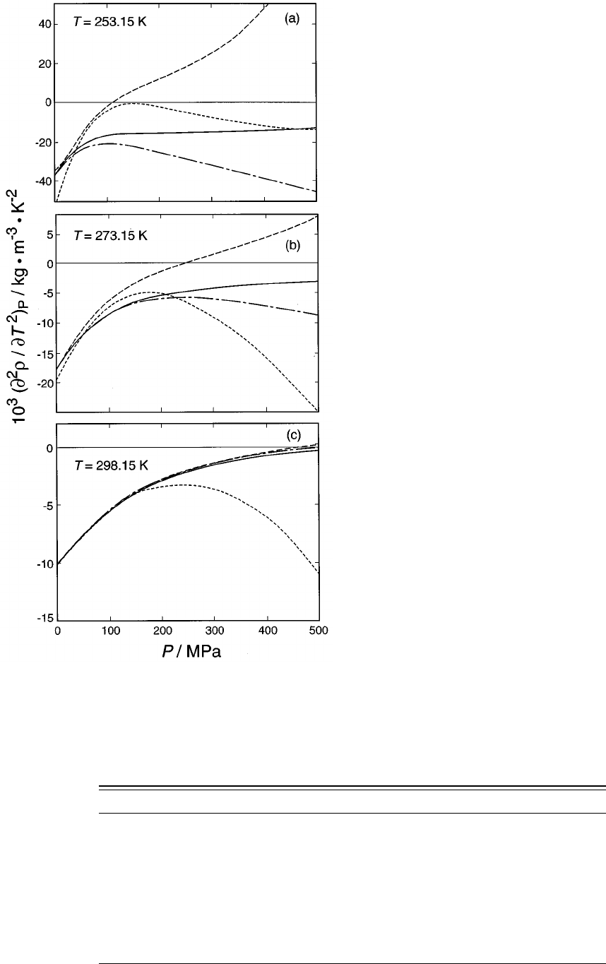
critical regime, reveals that the agreement between the vari-
ous formulations, in general, is better than that shown in Fig.
22.
Another estimate of the reliability of the Debye–Hu
¨
ckel
coefficients is obtained by comparing values derived from an
independent formulation of the dielectric constant, such as
that of Archer and Wang,
13
which used a different equation
of state. Such a comparison is made in Table 18.
We find that in the range of liquid water up to 473 K, the
values for A
V
agree on the level of 2%–3%, while those for
A
H
agree to within 1%, except at 273 K, where the differ-
ences are from 3% to 6%. These differences are slightly
larger than those for the first pressure derivative of the di-
electric constant, Table 13, thus confirming that the equation
of state contributes to the uncertainty of the Debye–Hu
¨
ckel
coefficients. In the supercritical regime, the spread is much
larger, especially for A
V
, where the difference between pre-
dictions from the two correlations is of the order of the value
itself at 773 K and 100 MPa. Since the values of the first
pressure derivative of the dielectric constant, according to
the two formulations, agree to within 4% at this state point
~Table 15!, the large additional uncertainty must be due to
the difference between the equations of state used.
The coefficient A
K
appears to be defined on a level of 25%
in the range up to 473 K, and somewhat better, within 10%,
in the supercritical range. This is roughly consistent with the
agreement of the second temperature derivative of the dielec-
tric constant displayed in Table 16.
The value of A
C
, of importance in heat capacity measure-
ments, is not well defined at 273 K. In the middle range,
298–473 K, the two formulations agree to its value to better
than 4%, and at supercritical temperatures to within 5%–
15%. The second temperature derivative of the dielectric
constant ~Table 14!, however, shows a smaller spread be-
tween these two formulations, consistent with the idea that
the equation of state makes an additional contribution to the
uncertainty of the Debye–Hu
¨
ckel coefficients. Comparisons
of the Debye–Hu
¨
ckel coefficients obtained from earlier cor-
relations can be found elsewhere.
98
FIG. 22. The second temperature derivative of the density, according to a
variety of high-quality equations of state....Ref. 100;----Ref. 101; full
curve, Ref. 19; -• -• - Ref. 14.
TABLE 18. Percentage difference of our predicted Debye–Hu
¨
ckel coefficient values from those of Archer and
Wang ~Ref. 13!.
T/K p/MPa A
f
A
V
A
H
A
K
A
C
273.150 0.1 20.002 4.09 23.38 31.6 23.5
273.150 100 20.091 20.09 26.82 26.5 69.4
298.144 0.1 20.056 3.54 20.80 20.0 20.41
298.144 50 20.117 1.50 0.17 24.2 1.33
298.144 200 20.041 23.70 0.61 10.8 23.73
373.124 0.101 325 20.044 22.63 0.92 217.3 2.41
373.124 100 0.003 0.61 1.66 25.08 4.11
473.110 100 0.409 0.49 1.16 28.70 22.37
673.102 100 20.162 1.64 0.38 2.03 5.01
773.071 100 1.44 7.37 6.74 10.3 13.2
11591159A FORMULATION FOR THE STATIC PERMITTIVITY OF WATER AND STEAM
J. Phys. Chem. Ref. Data, Vol. 26, No. 4, 1997
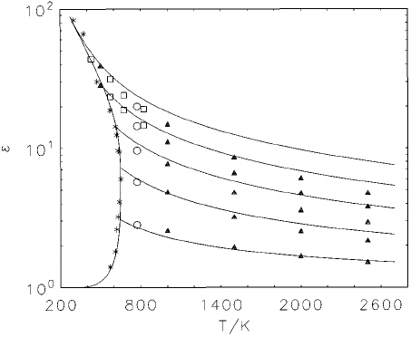
8. High-Temperature Behavior
and Extrapolation
The behavior of the dielectric constant of water at high
temperature and in the supercritical regime is of importance
to geological and hydrothermal applications. The upper limit
of the data is presently at 873 K, while information at even
higher temperatures is urgently desired. Experiments under
these conditions, however, become more arduous as tem-
perature and pressure increase, while, on the other hand, the
molecular behavior is expected to become simpler because
of the diminishing importance of hydrogen bonding. Thus
there have been several theoretical efforts at describing the
supercritical regime in such a way that extrapolation to
higher temperatures becomes feasible. We have described
some of these efforts in Section 2.2, and have seen that their
predictions are reasonably consistent with the experimental
data available well above the critical point ~Table 1!, and
must therefore also be consistent with our formulation in the
range where data exist. Table 1 bears this out. It is also clear
from Table 1 that the theoretical predictions, on extrapola-
tion, have the dielectric constant decline at a faster rate than
the extrapolation from our formulation.
As also discussed in Section 2.2, computer simulation has
recently been making substantial inroads into the realm of
supercritical water. A large body of information is now
available for the dielectric constant of water according to the
SPC/E model, see Sec. 2.2 and Refs. 51 and 53–57.
In Fig. 23, we compare the high-temperature simulation
results with our formulation in the range where data exist as
well as at higher temperatures. The simulation results are
shown along selected isochores in the density range up to
1000 kg m
2 3
and at temperatures up to 2600 K. The solid
lines give the results of our correlation along the same iso-
chores in the same regime.
There is an obvious mismatch in slope between simulation
and formulation, the simulation data declining more steeply
with temperature than the formulation, especially at the
higher densities. This mismatch, however, already occurs in
the range below 873 K, where experimental data exist, and
may, therefore, reflect the approximate character of the
SPC/E model. Had we chosen to follow the SPC/E results,
we would have had an appreciable departure from the avail-
able supercritical experimental data. It is no surprise that the
SPC/E model is not accurate at high densities.
58
In addition,
SPC/E predictions must be expected to deviate as well at
very low densities, since SPC/E does not take into account
the polarizability of the water molecule, and assumes an ef-
fective dipole moment higher than that of isolated water mol-
ecules. Given the low values of the dielectric constant in the
dilute steam phase, such departures would not be visible on
the scale of Fig. 23.
It is obvious that our correlation extrapolates smoothly to
high temperatures. In the absence of data, it is impossible to
assess the uncertainty of the values produced. In using the
formulation for predictions of the dielectric costant values as
a function of pressure and temperature in that range, one
needs to realize that the range of validity of the Wagner
equation of state does not exceed 1273 K. This limitation is
not a concern when density and temperature are used as vari-
ables.
9. Conclusions
A new formulation of the dielectric constant of water and
steam, including supercooled and supercritical states has
been presented; pressure and temperature derivatives of the
dielectric constant and the associated Debye–Hu
¨
ckel coeffi-
cients have been calculated, and their reliability has been
evaluated. The formulation is based on selected and carefully
evaluated experimental data, some of which has recently
been acquired. Use has been made of the most recent formu-
lation of the equation of state of water and steam which is
based on the new temperature scale ITS-90.
At the end of a large project such as the present one,
authors tend to focus on the deficits more than on the
achievements. The lack of a sound physical basis for formu-
lating the behavior of the dielectric constant of water and
steam is painfully clear, notwithstanding a long and concen-
trated effort by some of the greatest minds in the field of
physical chemistry. Although computer simulation has
shown major improvement, and offers promise, especially at
high temperatures, it is not yet quite at the cutting edge.
Data gaps and discrepancies between the two most impor-
tant data sources
8,12,48,49
affect the liquid range above 373 K,
and most of the supercritical regime. Except for the limited
range of liquid water at atmospheric pressure, the derivatives
of the dielectric constant, especially the second ones, are
known with quite limited reliability. In addition to the uncer-
tainty of the dielectric constant derivatives, that of the
FIG. 23. Comparison of high-temperature computer simulation data for the
SPC/E model with our correlation. Isochores are for 1.0, 0.8, 0.6, 0.4, and
0.2 kg dm
23
, respectively, from top to bottom. s, Wallqvist ~Ref. 58!; h,
Mountain ~Ref. 58!; m, Neumann ~Ref. 57!; !, simulated coexistence curve,
Guissani ~Ref. 56!; solid curves: the present correlation.
11601160 FERNANDEZ
ET AL.
J. Phys. Chem. Ref. Data, Vol. 26, No. 4, 1997
equation-of-state derivatives contributes to the uncertainty of
the Debye–Hu
¨
ckel coefficients. Particularly troublesome is
the region of supercooled water, in which the second deriva-
tives of the equation of state tend to develop unwanted os-
cillations.
It is, nevertheless, gratifying to see that the worst-case
scenario, based on estimates of uncertainty of experimental
dielectric constant and equation-of-state derivatives, does not
appear to play out. A comparison of the Debye–Hu
¨
ckel co-
efficients of two independent formulations, based on high
quality, but different equations of state, give values of these
coefficients that are generally close except near the edges of
the range where data are available.
Further progress will require new dielectric constant data
in the liquid above the boiling point and in the supercritical
regime. Although these are challenging regimes because of
the substantial conductivity of water in the denser states, and
the impurity effects due to corrosion, progress may be pos-
sible if use is made of the new flow methods that are begin-
ning to dominate high-temperature aqueous physical chem-
istry.
We are not optimistic that the data situation in the super-
cooled liquid can be easily remedied. The dielectric constant
measurements in that range require very small samples, or
the use of emulsifiers, in order to extend the lifetime of the
metastable state. The newest equations of state have already
been pushed to the limit as far as representing the available
data, but the higher derivatives of multiparameter equations
of state will always have reduced reliability near the edge of
the experimental range.
Note added in proof. After completion of the manuscript,
the following paper was brought to our attention: W. J. Elli-
son, K. Lamkaouchi, and J.-M. Moreau, J. Mol. Liquids 68,
171 ~1996!. This paper reviews and correlates the dielectric
data and their frequency dependence for liquid water be-
tween the freezing point and the boiling point.
10. Acknowledgments
We are greatly indebted to Dr. R. F. Kayser, Chief of the
Physical and Chemical Properties Division at NIST, for his
staunch support of the project throughout its long duration.
We have had several consultations with Professor E. U.
Franck. Professor M. Neumann advised on high-temperature
extrapolations. Dr. S. Penoncello was involved in early
stages of the project. We thank J. S. Gallagher for producing
Table 20, and for providing Fig. 22, and Dr. R. D. Mountain
for the comparison of computer simulation results with the
new formulation, Fig. 23. Dr. A. H. Harvey has served as a
thorough and critical reviewer and has carefully checked
many of the numerical results. Dr. A. Anderko reviewed the
manuscript and recommended developing auxiliary equa-
tions for the dielectric constant of saturated water and steam.
Dr. D. A. Archer provided useful criticism.
11. Appendix
Values of the dielectric constant of water and steam at
selected integer values of temperature, in Kelvin ~ITS-90!
and of pressure, in MPa, are presented in Table 19. Values in
ranges where no data exist are indicated in italics. Entries in
bold-face are in supercooled water. Liquid-vapor and fluid-
solid phase boundaries are indicated by horizontal bars. In
Table 20, dielectric constant values are tabulated with den-
sity and temperature as entries. This is the preferred repre-
sentation for the supercritical regime, and also facilitates
comparison with computer simulation results.
11611161A FORMULATION FOR THE STATIC PERMITTIVITY OF WATER AND STEAM
J. Phys. Chem. Ref. Data, Vol. 26, No. 4, 1997

TABLE 19. Dielectric constant of water and steam as a function of temperature and pressure.
p/MPa
T/K 0.1 1 2 5 10 20 30 40 50 60 70
260 93.41
265 91.26 —— —— ——
270 89.18
—— —— —— —— —— —— —— 91.25 91.64 92.04
275 87.16 87.20 87.24 87.36 87.57 87.97 88.38 88.77 89.16 89.55 89.93
280 85.19 85.23 85.27 85.39 85.59 85.98 86.37 86.76 87.14 87.51 87.89
285 83.27 83.30 83.34 83.46 83.65 84.04 84.42 84.80 85.17 85.53 85.89
290 81.39 81.42 81.46 81.57 81.76 82.14 82.51 82.88 83.24 83.60 83.96
295 79.55 79.58 79.62 79.73 79.92 80.29 80.65 81.01 81.37 81.72 82.06
300 77.75 77.78 77.82 77.93 78.11 78.48 78.83 79.19 79.54 79.88 80.22
305 75.99 76.02 76.06 76.17 76.35 76.71 77.06 77.41 77.75 78.09 78.42
310 74.27 74.30 74.33 74.44 74.62 74.98 75.32 75.67 76.01 76.34 76.67
315 72.58 72.61 72.65 72.76 72.93 73.28 73.63 73.97 74.30 74.63 74.96
320 70.93 70.97 71.00 71.11 71.28 71.63 71.97 72.31 72.64 72.96 73.28
325 69.32 69.36 69.39 69.50 69.67 70.02 70.35 70.69 71.01 71.34 71.65
330 67.75 67.78 67.82 67.92 68.09 68.44 68.77 69.10 69.43 69.75 70.06
335 66.21 66.24 66.27 66.38 66.55 66.89 67.23 67.55 67.88 68.19 68.51
340 64.70 64.73 64.77 64.87 65.04 65.38 65.72 66.04 66.36 66.68 66.99
345 63.23 63.26 63.30 63.40 63.57 63.91 64.24 64.56 64.88 65.20 65.51
350 61.79 61.82 61.85 61.96 62.13 62.47 62.80 63.12 63.44 63.75 64.06
355 60.38 60.41 60.45 60.55 60.72 61.06 61.39 61.71 62.03 62.34 62.65
360 59.00 59.03 59.07 59.17 59.34 59.68 60.01 60.33 60.65 60.96 61.27
365 57.66 57.69 57.72 57.83 58.00 58.34 58.67 58.99 59.30 59.61 59.92
370 56.34
56.37 56.41 56.51 56.68 57.02 57.35 57.67 57.99 58.30 58.60
375 1.006 55.09 55.12 55.22 55.40 55.74 56.07 56.39 56.70 57.01 57.32
380 1.006 53.83 53.86 53.97 54.14 54.48 54.81 55.13 55.45 55.76 56.06
390 1.005 51.39 51.43 51.53 51.71 52.05 52.38 52.71 53.03 53.34 53.64
400 1.005 49.06 49.10 49.21 49.39 49.73 50.07 50.39 50.71 51.02 51.33
410 1.005 46.84 46.87 46.98 47.16 47.51 47.85 48.18 48.50 48.82 49.12
420 1.005 44.70 44.74 44.85 45.04 45.39 45.74 46.07 46.39 46.71 47.02
430 1.004 42.66 42.70 42.81 43.00 43.36 43.71 44.05 44.38 44.70 45.01
440 1.004 40.70 40.74 40.85 41.05 41.42 41.77 42.12 42.45 42.77 43.09
450 1.004 38.81
38.85 38.97 39.17 39.55 39.92 40.27 40.61 40.93 41.25
460 1.004 1.041 37.04 37.17 37.37 37.76 38.14 38.50 38.84 39.17 39.50
470 1.004 1.039 35.30 35.43 35.64 36.04 36.43 36.80 37.15 37.49 37.82
480 1.004 1.038 33.61
33.75 33.97 34.39 34.79 35.17 35.53 35.87 36.21
490 1.003 1.036 1.078 32.13 32.36 32.79 33.21 33.60 33.97 34.32 34.66
500 1.003 1.034 1.074 30.55 30.79 31.25 31.68 32.09 32.47 32.84 33.18
525 1.003 1.031 1.066 26.79
27.07 27.61 28.09 28.54 28.96 29.35 29.73
550 1.003 1.028 1.059 1.177 23.53 24.18 24.75 25.26 25.73 26.17 26.58
575 1.002 1.026 1.054 1.154 20.00
20.87 21.58 22.19 22.74 23.23 23.68
600 1.002 1.024 1.049 1.137 1.365 17.50 18.48 19.25 19.90 20.48 20.99
625 1.002 1.022 1.045 1.124 1.306 13.62
15.28 16.35 17.18 17.87 18.47
650 1.002 1.020 1.041 1.112 1.267 2.066 11.58 13.37 14.50 15.36 16.08
675 1.002 1.019 1.038 1.103 1.238 1.744 5.359 10.05 11.78 12.91 13.79
700 1.002 1.017 1.036 1.095 1.214 1.603 2.666 6.260 8.963 10.50 11.59
725 1.002 1.016 1.033 1.088 1.195 1.514 2.158 3.772 6.298 8.184 9.494
750 1.002 1.015 1.031 1.082 1.179 1.452 1.921 2.831 4.424 6.183 7.600
775 1.001 1.014 1.029 1.076 1.166 1.404 1.775 2.396 3.405 4.726 6.031
800 1.001 1.013 1.027 1.071 1.154 1.365 1.674 2.142 2.844 3.791 4.854
825 1.001 1.013 1.026 1.067 1.143 1.334 1.598 1.973 2.501 3.201 4.029
850 1.001 1.012 1.024 1.063 1.134 1.307 1.538 1.850 2.269 2.810 3.459
875 1.001 1.011 1.023 1.059 1.126 1.284 1.489 1.757 2.102 2.536 3.056
900 1.001 1.011 1.022 1.056 1.118 1.265 1.449 1.682 1.975 2.335 2.761
950 1.001 1.010 1.020 1.050 1.105 1.232 1.385 1.570 1.793 2.057 2.363
1000 1.001 1.009 1.018 1.046 1.095 1.206 1.336 1.489 1.668 1.874 2.108
1050 1.001 1.008 1.016 1.041 1.086 1.184 1.298 1.428 1.576 1.744 1.931
1100 1.001 1.007 1.015 1.038 1.078 1.167 1.266 1.379 1.505 1.646 1.801
1150 1.001 1.007 1.014 1.035 1.072 1.151 1.240 1.339 1.449 1.569 1.701
1200 1.001 1.006 1.013 1.032 1.066 1.139 1.219 1.307 1.403 1.508 1.622
11621162 FERNANDEZ
ET AL.
J. Phys. Chem. Ref. Data, Vol. 26, No. 4, 1997

TABLE 19. Dielectric constant of water and steam as a function of temperature and pressure—Continued
p/MPa
T/K 80 100 150 200 250 300 350 1400 1450 1500 1000
260 —— 99.66 101.5 103.3 105.0 106.6 108.2 109.8
265 —— 95.41 97.31 99.11 100.8 102.5 104.1 105.7 107.2 ——
270 92.43 93.19 95.04 96.80 98.48 100.1 101.7 103.2 104.7 106.2
275 90.31 91.05 92.85 94.55 96.19 97.77 99.30 100.8 102.3 103.7
280 88.25 88.98 90.72 92.38 93.97 95.51 97.00 98.45 99.87 101.3
285 86.25 86.96 88.65 90.27 91.82 93.32 94.77 96.18 97.56 98.91
290 84.30 84.99 86.65 88.22 89.74 91.19 92.61 93.98 95.32 96.64
295 82.41 83.08 84.70 86.24 87.71 89.14 90.51 91.85 93.16 94.44
300 80.56 81.22 82.80 84.31 85.75 87.14 88.48 89.79 91.06 92.31 ——
305 78.75 79.40 80.96 82.43 83.85 85.20 86.52 87.79 89.04 90.25 101.3
310 76.99 77.63 79.16 80.61 82.00 83.33 84.61 85.86 87.08 88.26 99.06
315 75.28 75.90 77.41 78.84 80.20 81.50 82.77 83.99 85.18 86.34 96.87
320 73.60 74.22 75.71 77.11 78.45 79.74 80.97 82.17 83.34 84.48 94.76
325 71.97 72.58 74.05 75.43 76.75 78.02 79.23 80.41 81.56 82.67 92.73
330 70.37 70.98 72.43 73.80 75.10 76.34 77.54 78.70 79.83 80.92 90.78
335 68.81 69.42 70.85 72.20 73.49 74.72 75.90 77.04 78.15 79.23 88.89
340 67.29 67.89 69.31 70.65 71.92 73.14 74.30 75.43 76.52 77.58 87.07
345 65.81 66.40 67.82 69.14 70.40 71.60 72.75 73.86 74.94 75.98 85.31
350 64.36 64.95 66.35 67.67 68.91 70.10 71.24 72.34 73.40 74.43 83.61
355 62.95 63.53 64.93 66.23 67.47 68.64 69.77 70.85 71.90 72.92 81.96
360 61.57 62.15 63.53 64.83 66.05 67.22 68.33 69.41 70.44 71.45 80.36
365 60.22 60.80 62.18 63.46 64.68 65.83 66.94 68.00 69.03 70.02 78.81
370 58.90 59.48 60.85 62.13 63.34 64.48 65.58 66.63 67.65 68.63 77.31
375 57.61 58.19 59.56 60.83 62.03 63.17 64.25 65.29 66.30 67.27 75.85
380 56.36 56.94 58.30 59.57 60.76 61.88 62.96 63.99 64.99 65.95 74.43
390 53.94 54.51 55.87 57.12 58.30 59.41 60.47 61.49 62.47 63.41 71.71
400 51.62 52.20 53.55 54.80 55.96 57.06 58.11 59.11 60.07 61.00 69.12
410 49.42 50.00 51.34 52.58 53.74 54.83 55.86 56.85 57.79 58.71 66.68
420 47.32 47.90 49.24 50.48 51.62 52.70 53.72 54.69 55.63 56.53 64.35
430 45.31 45.89 47.24 48.47 49.61 50.67 51.68 52.65 53.57 54.45 62.13
440 43.39 43.98 45.33 46.55 47.69 48.74 49.74 50.69 51.60 52.48 60.03
450 41.56 42.15 43.51 44.73 45.86 46.91 47.90 48.84 49.74 50.60 58.02
460 39.81 40.40 41.77 42.99 44.11 45.16 46.14 47.07 47.96 48.81 56.11
470 38.13 38.74 40.11 41.33 42.45 43.49 44.46 45.38 46.26 47.10 54.28
480 36.53 37.14 38.52 39.75 40.87 41.90 42.86 43.78 44.64 45.47 52.55
490 34.99 35.61 37.01 38.24 39.35 40.38 41.34 42.24 43.10 43.92 50.89
500 33.52 34.15 35.56 36.79 37.91 38.93 39.89 40.78 41.63 42.44 49.30
525 30.08 30.75 32.20 33.46 34.57 35.59 36.53 37.41 38.24 39.03 45.64
550 26.96 27.67 29.18 30.46 31.59 32.60 33.53 34.40 35.22 35.99 42.38
575 24.10 24.86 26.46 27.77 28.91 29.92 30.85 31.71 32.51 33.26 39.45
600 21.46 22.29 23.98 25.34 26.49 27.51 28.44 29.28 30.07 30.82 36.82
625 19.00 19.92 21.72 23.13 24.31 25.34 26.26 27.10 27.88 28.61 34.45
650 16.69 17.72 19.65 21.12 22.32 23.36 24.29 25.13 25.90 26.62 32.31
675 14.51 15.67 17.76 19.28 20.52 21.57 22.50 23.33 24.10 24.81 30.36
700 12.44 13.75 16.01 17.60 18.87 19.93 20.87 21.70 22.46 23.17 28.60
725 10.49 11.97 14.40 16.06 17.36 18.44 19.38 20.21 20.97 21.67 26.98
750 8.702 10.34 12.93 14.65 15.97 17.07 18.01 18.85 19.60 20.30 25.51
775 7.145 8.857 11.58 13.35 14.70 15.81 16.76 17.60 18.35 19.04 24.15
800 5.872 7.562 10.35 12.17 13.54 14.66 15.61 16.45 17.20 17.88 22.91
825 4.894 6.468 9.246 11.09 12.47 13.60 14.55 15.39 16.14 16.82 21.76
850 4.169 5.571 8.263 10.10 11.49 12.62 13.58 14.41 15.16 15.83 20.70
875 3.637 4.852 7.399 9.215 10.60 11.73 12.68 13.51 14.25 14.92 19.71
900 3.241 4.284 6.647 8.416 9.787 10.91 11.85 12.68 13.41 14.08 18.80
950 2.707 3.477 5.441 7.066 8.374 9.460 10.39 11.20 11.92 12.57 17.15
1000 2.369 2.956 4.557 6.003 7.218 8.250 9.143 9.930 10.63 11.27 15.72
1050 2.138 2.601 3.908 5.172 6.280 7.244 8.091 8.845 9.524 10.14 14.45
1100 1.970 2.347 3.427 4.523 5.520 6.409 7.203 7.918 8.567 9.160 13.34
1150 1.843 2.158 3.063 4.012 4.905 5.717 6.454 7.127 7.742 8.309 12.35
1200 1.744 2.011 2.781 3.606 4.403 5.143 5.823 6.451 7.031 7.569 11.47
11631163A FORMULATION FOR THE STATIC PERMITTIVITY OF WATER AND STEAM
J. Phys. Chem. Ref. Data, Vol. 26, No. 4, 1997

TABLE 20. Dielectric constant of water and steam as a function of temperature and density.
r
/kg m
2 3
T/K
50 100 150 200 250 300 350 400 450 500
580 1.379
600 1.367
620 1.355 1.822
640 1.344 1.795 2.371 10.21
660 1.334 1.770 2.325 3.012 3.834 4.790 5.878 7.090 8.417 9.850
680 1.325 1.746 2.282 2.943 3.734 4.653 5.698 6.863 8.138 9.516
700 1.316 1.724 2.242 2.880 3.642 4.527 5.533 6.653 7.881 9.208
750 1.296 1.675 2.154 2.741 3.439 4.250 5.170 6.195 7.319 8.534
800 1.278 1.634 2.079 2.622 3.268 4.017 4.866 5.811 6.848 7.971
850 1.263 1.597 2.014 2.521 3.122 3.818 4.606 5.484 6.448 7.491
900 1.250 1.565 1.957 2.433 2.995 3.646 4.382 5.203 6.103 7.079
950 1.238 1.537 1.907 2.355 2.884 3.495 4.187 4.957 5.802 6.719
1000 1.227 1.512 1.863 2.287 2.786 3.362 4.014 4.740 5.537 6.402
1050 1.218 1.489 1.823 2.225 2.698 3.244 3.861 4.548 5.302 6.121
1100 1.209 1.469 1.787 2.170 2.620 3.138 3.724 4.376 5.092 5.869
1150 1.201 1.450 1.755 2.120 2.549 3.042 3.600 4.221 4.903 5.643
1200 1.194 1.433 1.725 2.075 2.484 2.956 3.488 4.081 4.731 5.438
Saturation
T/K→ 577.95 616.99 634.68 642.96 646.25 647.07 647.05 646.11 643.27 637.55
e
1.381 1.826 2.384 3.074 3.907 4.885 6.003 7.260 8.670 10.26
r
/kg m
2 3
T/K
550 600 650 700 750 800 850 900 950 1000
300 78.03
320 71.80
340 66.34
360 61.53
380 57.29
400 49.92 53.53
420 46.71 50.19
440 43.87 47.21
460 38.24 41.33 44.54
480 36.11 39.07 42.15
500 31.44 34.19 37.04 40.00
520 29.84 32.47 35.20 38.05
540 25.94 28.39 30.93 33.55 36.29
560 22.45 24.74 27.09 29.52 32.05 34.69
580 19.32 21.45 23.65 25.91 28.25 30.68 33.23
600 16.52 18.50 20.54 22.65 24.83 27.08 29.43 31.89
620 14.02 15.85 17.75 19.72 21.75 23.85 26.02 28.28 30.67
640 11.81 13.48 15.24 17.07 18.96 20.92 22.94 25.04 27.23 29.54
660 11.38 12.99 14.68 16.44 18.27 20.16 22.11 24.14 26.26 28.49
680 10.99 12.54 14.17 15.87 17.63 19.46 21.35 23.31 25.37 27.53
700 10.63 12.12 13.70 15.34 17.04 18.81 20.64 22.54 24.53 26.64
750 9.835 11.21 12.66 14.17 15.75 17.38 19.08 20.85 22.70 24.66
800 9.173 10.45 11.79 13.19 14.66 16.18 17.76 19.42 21.15 22.99
850 8.610 9.797 11.05 12.36 13.73 15.15 16.64 18.19 19.83 21.56
900 8.125 9.237 10.41 11.64 12.93 14.27 15.67 17.14 18.68 20.32
950 7.702 8.748 9.853 11.01 12.23 13.50 14.82 16.21 17.68 19.24
1000 7.330 8.318 9.363 10.46 11.61 12.81 14.07 15.39 16.79 18.28
1050 7.000 7.937 8.928 9.971 11.06 12.21 13.41 14.67 16.00 17.42
1100 6.705 7.596 8.539 9.532 10.57 11.67 12.81 14.02 15.29 16.66
1150 6.439 7.289 8.188 9.137 10.13 11.18 12.28 13.43 14.66 15.97
1200 6.199 7.011 7.871 8.779 9.734 10.74 11.79 12.90 14.08 15.34
Saturation
T/K→ 628.82 616.34 599.78 578.91 553.30 522.40 485.36 440.64 384.39
e
12.06 14.12 16.53 19.36 22.80 27.11 32.73 40.56 52.72
11641164 FERNANDEZ
ET AL.
J. Phys. Chem. Ref. Data, Vol. 26, No. 4, 1997
12. References
1
P. Debye and E. Hu
¨
ckel, Phys. Z. 24, 185 ~1923!.
2
M. Born, Z. Phys. 1,45~1920!.
3
D. P. Ferna
´
ndez, Y. V. Mulev, A. R. H. Goodwin, and J. M. H. Levelt
Sengers, J. Phys. Chem. Ref. Data 24,33~1995!.
4
A. S. Quist and W. L. Marshall, J. Phys. Chem. 9, 3165 ~1965!.
5
H. C. Helgeson and D. H. Kirkham, Am. J. Sci. 274, 1089 ~1974!.
6
H. I. Oshry, Ph.D. dissertation, University of Pittsburgh ~1949!.
7
B. B. Owen, R. C. Miller, C. E. Milner, and H. L. Cogan, J. Phys. Chem.
Ref. Data 65, 2065 ~1961!.
8
K. Heger, Ph.D. dissertation, University of Karlsruhe ~1969!.
9
J. H. Keenan, F. G. Keyes, P. G. Hill, and J. G. Moore, Steam Tables
~Wiley, New York, 1969!.
10
D. J. Bradley and K. S. Pitzer, J. Phys. Chem. 83, 1599 ~1979!.
11
M. Uematsu and E. U. Franck, J. Phys. Chem. Ref. Data 9, 1291 ~1980!.
12
K. Heger, M. Uematsu, and E. U. Franck, Ber. Bunsenges. Phys. Chem.
84, 758 ~1980!.
13
D. G. Archer and P. Wang, J. Phys. Chem. Ref. Data 19, 371 ~1990!.
14
P. G. Hill, J. Phys. Chem. Ref. Data 19, 1233 ~1990!.
15
J. W. Johnson and D. Norton, Am. J. Sci. 291, 541 ~1991!.
16
D. P. Ferna
´
ndez, A. R. H. Goodwin, and J. M. H. Levelt Sengers, Int. J.
Thermophys. 16, 929 ~1995!.
17
Yu. V. Mulev, S. N. Smirnov, and M. R. Muchailov, Teploenergetica ~in
press, 1996!.
18
H. Preston-Thomas, Metrologia 27,3~1990!.
19
W. Wagner and A. Pruss, private communication ~1995!; J. Phys. Chem.
Ref. Data ~submitted!.
20
Release on the IAPWS Formulation 1995 for the Thermodynamic Prop-
erties of Ordinary Water Substance for General and Scientific Use, Fre-
dericia, Denmark, September 1996, to be obtained from the Executive
Secretary of IAPWS, Dr. R. B. Dooley, Electric Power Research Institute,
3412 Hillview Avenue, Palo Alto, CA 94304-1395.
21
R. J. Speedy and C. A. Angell, J. Chem. Phys. 65, 851 ~1976!.
22
I. M. Hodge and C. A. Angell, J. Chem. Phys. 68, 1363 ~1978!.
23
J. B. Hasted and M. Shahidi, Nature 262, 777 ~1976!.
24
D. Bertolini, M. Cassettari, and G. Salvetti, J. Chem. Phys. 76, 3285
~1982!.
25
G. Stell and J. S. Ho”ye, Phys. Rev. Lett. 33, 1268 ~1974!.
26
D. Bedeaux and P. Mazur, Physica 67,23~1973!.
27
T. Doiron and H. Meyer, Phys. Rev. B17, 2141 ~1979!.
28
B. J. Thijsse, T. Doiron, and J. M. H. Levelt Sengers, Chem. Phys. Lett.
72, 546 ~1980!.
29
M. H. W. Chan, Phys. Rev. B 21, 1187 ~1980!.
30
M. W. Pestak and M. H. W. Chan, Phys. Rev. Lett. 46, 943 ~1981!.
31
H. A. Lorentz, Theory of Electrons ~Leipzig, 1909!.
32
C. J. F. Bo
¨
ttcher, Theory of Electric Polarization, 2nd ed., revised by O.
C. Van Belle, P. Bordewijk, and A. Rip ~Elsevier, Amsterdam, 1973!.
33
P. Debye, Phys. Z. 13,97~1912!.
34
R. P. Bell, Trans. Faraday Soc. 27, 797 ~1931!.
35
L. Onsager, J. Am. Chem. Soc. 58, 1486 ~1936!.
36
J. G. Kirkwood, J. Chem. Phys. 7, 911 ~1939!.
37
F. E. Harris and B. J. Alder, J. Chem. Phys. 21, 1031 ~1953!.
38
H. Fro
¨
hlich, Physica 22, 898 ~1956!.
39
R. H. Cole, J. Chem. Phys. 27,33~1957!.
40
N. E. Hill, Trans. Faraday Soc. 59, 344 ~1963!.
41
J. B. Hasted, Aqueous Dielectrics ~Chapman and Hall, London, 1973!.
42
H. Fro
¨
hlich, Theory of Dielectrics ~Oxford University, Oxford, 1958!.
43
J. B. Hasted, in Water, A Comprehensive Treatise, Vol. 1, Chap. 7, edited
by F. Franks ~Plenum, New York, 1972!.
44
O. A. Nabokov and Yu. A. Lyubimov, J. Struct. Chem. 27, 731 ~1986!.
45
G. Oster and J. G. Kirkwood, J. Chem. Phys. 11, 175 ~1943!.
46
E. U. Franck, S. Rosenzweig, and M. Christoforakos, Ber. Bunsenges.
Phys. Chem. 94, 199 ~1990!.
47
G. N. Patey, D. Levesque, and J. J. Weis, Mol. Phys. 38, 219 ~1979!.
48
R. Deul, Ph.D. dissertation, University of Karlsruhe ~1984!.
49
R. Deul and E. U. Franck, Ber. Bunsenges. Phys. Chem. 95, 847 ~1991!.
50
S. Goldman, C. Joslin, and E. A. Wasserman, J. Phys. Chem. 98, 6231
~1994!.
51
H. J. C. Berendsen, J. R. Grigera, and T. P. Straatsma, J. Phys. Chem. 91,
6269 ~1987!.
52
E. A. Wasserman, B. J. Wood, and J. Brodholt, Ber. Bunsenges. Phys.
Chem. 98, 906 ~1994!.
53
G. P. Johari, J. Chem. Phys. 80, 4413 ~1984!.
54
M. Neumann, J. Chem. Phys. 82, 5663 ~1985!.
55
M. Sprik, J. Chem. Phys. 95, 6762 ~1991!.
56
Y. Guissani and B. Guillot, J. Chem. Phys. 98, 8221 ~1993!.
57
M. Neumann, Proceedings of the 12th ICPWS, Orlando, FL, 1994, edited
by H. J. White, Jr., J. V. Sengers, D. Neumann, and J. C. Bellows ~Begell
House, New York, 1995!.
58
R. D. Mountain and A. Wallqvist, NISTIR 5778 ~1996!.
59
P. Schiebener, J. Straub, J. M. H. Levelt Sengers, and J. S. Gallagher, J.
Phys. Chem. Ref. Data 19, 677 ~1990!.
60
W. L. Lees, Ph.D. dissertation, Harvard University ~1949!.
61
C. E. Milner, Ph.D. dissertation, Yale University ~1955!.
62
H. L. Cogan, Ph.D. dissertation, Yale University ~1958!.
63
E. W. Rusche, Ph.D. dissertation, New Mexico University ~1966!.
64
R. L. Kay, G. A. Vidulich, and K. S. Pribadi, J. Phys. Chem. 73, 445
~1969!.
65
Yu. M. Lukashov, Ph.D. dissertation, Moscow Power Institute ~1981!.
66
G. C. Åkerlo
¨
f, J. Am. Chem. Soc. 54, 4125 ~1932!.
67
P. Albright, J. Am. Chem. Soc. 50, 2098 ~1937!.
68
P. S. Albright and L. J. Gosting, J. Am. Chem. Soc. 68, 1061 ~1946!.
69
F. H. Drake, G. W. Pierce, and M. T. Dow, Phys. Rev. 35, 613 ~1930!.
70
L. A. Dunn and R. H. Stokes, Trans. Faraday Soc. 65, 2906 ~1969!.
71
J. K. Fogo, S. W. Benson, and C. S. Copeland, J. Chem. Phys. 22, 209
~1954!.
72
T. E. Gier and H. S. Young, as reported by A.W. Lawson and A.J. Hughes
in High Pressure Physics and Chemistry, Vol. I, edited by R. S. Bradley
~Academic, New York, 1963!.
73
B. P. Golubev, Ph.D. ~Doctor! dissertation, Moscow Power Institute
~1978!.
74
E. H. Grant, T. J. Buchanan, and H. F. Cook, J. Chem. Phys. 26, 156
~1956!.
75
F. E. Harris, E. W. Haycock, and B. J. Alder, J. Chem. Phys. 21, 1943
~1953!; J. Phys. Chem. 57, 978 ~1953!.
76
U. Kaatze and V. Uhlendorf, Z. Phys. Chem. ~Neue Folge! 126, 151
~1981!.
77
Yu. M. Lukashov, B. P. Golubev, and F. B. Ripol-Saragosi, Teploenerge-
tika 22-6,79~1975!.
78
C. G. Malmberg and A. A. Maryott, J. Res. Natl. Bur. Stand. 56,1~1956!.
79
M. R. Muchailov, Ph.D. ~Candidate! dissertation, Moscow Power Institute
~1988!.
80
B. K. P. Scaife, Proc. Phys. Soc. London B68, 790 ~1955!.
81
E. Schadow and R. Steiner, Z. Phys. Chem. ~Neue Folge! 66, 105 ~1969!.
82
K. R. Srinivasan, Ph.D. dissertation, Carnegie-Mellon University ~1973!.
83
K. R. Srinivasan and R. L. Kay, J. Chem. Phys. 60, 3645 ~1974!.
84
E. P. Svistunov, B. P. Golubev, and S. N. Smirnov, Teploenergetika 21-6,
69 ~1974!.
85
T. Tyssul Jones and R. M. Davis, Philos. Mag. 28, 307 ~1939!.
86
G. A. Vidulich and R. L. Kay, J. Phys. Chem. 66, 383 ~1962!.
87
G. A. Vidulich, D. F. Evans, and R. L. Kay, J. Phys. Chem. 71, 656
~1967!.
88
J. Wyman and E. N. Ingalls, J. Am. Chem. Soc. 60, 1182 ~1938!.
89
J. Wyman, Phys. Rev. 35, 623 ~1930!.
90
E. R. Cohen and B. N. Taylor, J. Phys. Chem. Ref. Data 17, 1195 ~1988!.
91
Report of Investigation, NIST Standard Reference Material 8535 ~Vienna
Standard Mean Ocean Water!, NIST Standard Reference Materials Pro-
gram, Gaithersburg, MD ~1992!.
92
C. G. Gray and K. E. Gubbins, Theory of Molecular Fluids, Vol. 1 ~Clar-
endon, Oxford, 1984!.
93
W. Wagner, Fortschr.-Ber. VDI-Z., Vol. 3 ~#39! VDI-Verlag, Du
¨
sseldorf
~1974!,p.39.
94
B. N. Taylor and C. E. Kuyatt, NIST Technical Note 1297 ~1994!.
95
J. M. H. Levelt Sengers, C. M. Everhart, G. Morrison, and K. S. Pitzer,
Chem. Eng. Commun. 47, 315 ~1986!.
11651165A FORMULATION FOR THE STATIC PERMITTIVITY OF WATER AND STEAM
J. Phys. Chem. Ref. Data, Vol. 26, No. 4, 1997
96
E. A. Guggenheim, Thermodynamics ~North-Holland, Amsterdam, Neth-
erlands, 1967!.
97
K. S. Pitzer, Activity Coefficients in Electrolyte Solutions, Chap. 3 ~CRC,
Boca Raton, FL, 1991!.
98
P. S. Z. Rogers and K. S. Pitzer, J. Phys. Chem. Ref. Data 11,15~1982!.
99
R. P. Breyer and B. R. Staples, J. Soln. Chem. 15, 749 ~1986!.
100
L. Haar, J. S. Gallagher, and G. S. Kell, NBS/NRC Steam Tables ~Hemi-
sphere, Washington, DC, 1984!.
101
A. Saul and W. Wagner, J. Phys. Chem. Ref. Data 18, 1537 ~1989!.
11661166 FERNANDEZ
ET AL.
J. Phys. Chem. Ref. Data, Vol. 26, No. 4, 1997
