Recommendation ITU-R P.527-4
(06/2017)
Electrical characteristics
of the surface of the Earth
P Series
Radiowave propagation

ii Rec. ITU-R P.527-4
Foreword
The role of the Radiocommunication Sector is to ensure the rational, equitable, efficient and economical use of the radio-
frequency spectrum by all radiocommunication services, including satellite services, and carry out studies without limit of
frequency range on the basis of which Recommendations are adopted.
The regulatory and policy functions of the Radiocommunication Sector are performed by World and Regional
Radiocommunication Conferences and Radiocommunication Assemblies supported by Study Groups.
Policy on Intellectual Property Right (IPR)
ITU-R policy on IPR is described in the Common Patent Policy for ITU-T/ITU-R/ISO/IEC referenced in Annex 1 of
Resolution ITU-R 1. Forms to be used for the submission of patent statements and licensing declarations by patent holders
are available from http://www.itu.int/ITU-R/go/patents/en where the Guidelines for Implementation of the Common Patent
Policy for ITU-T/ITU-R/ISO/IEC and the ITU-R patent information database can also be found.
Series of ITU-R Recommendations
(Also available online at http://www.itu.int/publ/R-REC/en)
Series
Title
BO
Satellite delivery
BR
Recording for production, archival and play-out; film for television
BS
Broadcasting service (sound)
BT
Broadcasting service (television)
F
Fixed service
M
Mobile, radiodetermination, amateur and related satellite services
P
Radiowave propagation
RA
Radio astronomy
RS
Remote sensing systems
S
Fixed-satellite service
SA
Space applications and meteorology
SF
Frequency sharing and coordination between fixed-satellite and fixed service systems
SM
Spectrum management
SNG
Satellite news gathering
TF
Time signals and frequency standards emissions
V
Vocabulary and related subjects
Note: This ITU-R Recommendation was approved in English under the procedure detailed in Resolution ITU-R 1.
Electronic Publication
Geneva, 2017
ITU 2017
All rights reserved. No part of this publication may be reproduced, by any means whatsoever, without written permission of ITU.

Rec. ITU-R P.527-4 1
RECOMMENDATION ITU-R P.527-4
Electrical characteristics of the surface of the Earth
(1978-1982-1992-2017)
Scope
This Recommendation gives methods to model the electrical characteristics of the surface of the Earth,
including pure water, sea water, ice, soil and vegetation cover, for frequencies up to 1 000 GHz, in a systematic
manner based on the evaluation of complex relative permittivity. In all cases conductivity can be calculated as
a function of frequency and temperature from these evaluations. Previous information on electrical
characteristics below 30 MHz in terms of permittivity and conductivity is retained in Appendix in view of its
association with Recommendations ITU-R P.368 and ITU-R P.832. The new modelling method is fully
compatible with this earlier information.
Keywords
Complex permittivity, conductivity, penetration depth, Earth’s surface, water, vegetation, soil, ice
The ITU Radiocommunication Assembly,
considering
a) that the electrical characteristics may be expressed by three parameters: magnetic
permeability, electrical permittivity, , and electrical conductivity,;
b) that the permeability of the Earth’s surface, , can normally be regarded as equal to the
permeability in a vacuum;
c) that the electrical properties of the Earth’s surface can be expressed by the complex
permittivity or, equivalently, by the real part and imaginary part of the complex permittivity;
d) that information on the variation of the penetration depth with frequency is needed;
e) that knowledge of the electrical characteristics of the Earthʼs surface is needed for several
purposes in propagation modelling, including ground-wave signal strength, ground reflection at a
terrestrial terminal, interference between aeronautical and/or space borne stations due to reflections
or scattering from the Earth's surface, and for Earth science applications;
f) that Recommendation ITU-R P.368 contains ground-wave propagation curves from 1 MHz
to 30 MHz for different ground conditions characterised by permittivity and electrical conductivity;
g) that Recommendation ITU-R P.832 contains a world atlas of ground electrical conductivity
for frequencies below 1 MHz,
recommends
that the information in Annex 1 be used to model the electrical characteristics of the surface of the
Earth.

2 Rec. ITU-R P.527-4
Annex 1
1 Introduction
This Annex provides prediction methods that predict the electrical characteristics of the following
Earth’s surfaces for frequencies up to 1 000 GHz:
– Water
– Sea (i.e. Saline) Water
– Dry and Wet Ice
– Dry and Wet Soil (combination of sand, clay, and silt)
– Vegetation (above and below freezing)
2 Complex permittivity
The characteristics of the Earth’s surface can be characterized by three parameters:
– the magnetic permeability, ,
– the electrical permittivity, , and
– the electrical conductivity
1
, .
Magnetic permeability is a measure of a material’s ability to support the formation of a magnetic field
within itself in response to an applied magnetic field; i.e. the magnetic flux density B divided by the
magnetic field strength H. Electrical permittivity is a measure of a materialʼs ability to oppose an
electric field; i.e. the electrical flux density D divided by the electrical field strength E. Electrical
conductivity is a measure of a materialʼs ability to conduct an electric current; i.e. the ratio of the
current density in the material to the electric field that causes the current flow.
Given an incident plane wave
, with radial frequency , time , magnetic
permeability , electrical permittivity , and electrical conductivity , the propagation wave number
vector
, has a magnitude given by
(1a)
The vacuum values of permittivity, permeability, and conductivity are:
– Vacuum Permittivity
(F/m)
– Vacuum Permeability
(N/A
2
)
– Vacuum Conductivity
(S/m)
It is convenient to define the relative permittivity,
, and the relative permeability,
, relative to
their vacuum values as follows:
– Relative Permittivity
– Relative Permeability
where and are the associated permittivity and permeability of the medium. This Recommendation
assumes =
, in which case
= 1.
1
It is called electrical conductivity to differentiate it from other conductivities such as thermal conductivity
and hydraulic conductivity. It is called hereinafter as conductivity.

Rec. ITU-R P.527-4 3
As shown in equation (1a) the wavenumber depends on both and , not either separately. Also
formulations of other physical parameters describing various radio wave propagation mechanisms
such as scattering cross section, reflection coefficients, and refraction angles, depend on values of
this combination. Furthermore, the square root of this combination is equivalent to the refractive
index formulation used in characterizing the troposphere and the ionosphere. The refractive index is
also used in characterizing different materials at the millimetre wave and optical frequency bands.
Accordingly, to simplify the formulations describing various propagation mechanisms and to
standardize terminologies of electrical characteristics at different frequency bands, the combination
is defined as the complex permittivity and used to describe the electrical characteristics of
substances.
While permittivity refers to ε, relative permittivity refers to ε
, and complex relative permittivity,
defined as
refers to:
(1b)
where may be complex.
In equation (1b),
is the real part of the complex permittivity, and
is the imaginary part of the
complex permittivity. The real part of the complex relative permittivity,
, is associated with the
stored energy when the substance is exposed to an electromagnetic field. The imaginary part of the
complex relative permittivity,
, influences energy absorption and is known as the loss factor. The
minus sign in equation (1b) is associated with an electromagnetic field having time dependence of
(is frequency in Hz, and is time in seconds). If the time dependence is
, the minus
(–) sign in equation (1b) is replaced by a plus (+) sign.
At frequencies up to 1 000 GHz, dissipation within the Earth’s surface is attributed to either
translational (conduction current) charge motion or vibrational (dipole vibration) charge motion, and
the imaginary part of the complex relative permittivity,
can be decomposed into two terms:
(2)
where
′′
represents the dissipation due to displacement current associated with dipole vibration, and
represents the dissipation due to conduction current.
Conduction current consists of the bulk translation movement of free charges and is the only current
at zero (i.e. dc) frequency. Conduction current is greater than displacement current at frequencies
below the transition frequency,
, and the displacement current is greater than the conduction current
at frequencies above the transition frequency,
. The transition frequency,
, defined as the
frequency where the conduction and displacement currents are equal, is:
(3)
For non-conducting (lossless) dielectric substances , and hence
. For some of those
substances, such as dry soil and dry vegetation,
, and hence
irrespective of the
frequency, which is the case considered in § 2.1.2.3 of Recommendation ITU-R P.2040. On the other
hand, for some other non-conducting substances, such as pure water and dry snow,
, and hence
,
equal zero only at zero frequency. Accordingly, § 2.1.2.3 of Recommendation ITU-R P.2040 cannot
be applied to those substances.
For conducting (lossy) dielectric substances, such as sea water and wet soil, the electrical conductivity
has finite values different than zero. Accordingly, as the frequency tends to zero, the imaginary part
of the complex relative permittivity of those substances tends to as it can be inferred from
equation (3). In this case, it is easier to work with the conductivity instead of the imaginary part of

4 Rec. ITU-R P.527-4
the complex relative permittivity which can be written from equation (2) after setting
= 0 as
follows:
(3a)
with
is the frequency in GHz. Generalizing the above formulation to other frequencies, as done
by equation (12) of Recommendation ITU-R P.2040, yields the sum of two terms: one term gives the
electrical conductivity and the other term accounts for the power dissipation associated with the
displacement current.
This Recommendation provides prediction methods for the real and imaginary parts of the complex
relative permittivity,
and
; and the accompanying example figures show trends of the real and
imaginary parts of the complex relative permittivity with frequency under different environmental
conditions.
2.1 Layered ground
The models in § 5 apply to homogeneous sub-surface soil; however, the sub-surface is rarely
homogeneous. Rather, it consists of multiple layers of different thicknesses and different electrical
characteristics that must be taken into account by introducing the concept of effective parameters to
represent the homogeneous soil. Effective parameters can be used with the homogeneous smooth
Earth ground-wave propagation curves of Recommendation ITU-R P.368.
3 Penetration depth
The extent to which the lower strata influence the effective electrical characteristics of the Earth’s
surface depends upon the penetration depth of the radio energy, , which is defined as the depth at
which the amplitude of the field strength of electromagnetic radiation inside a material falls to 1/e
(about 37%) of its original value at (or more properly, just beneath) the surface. The penetration
depth, , in a homogeneous medium of complex relative permittivity
(
) is given by:
(m) (4)
where is the wavelength in metres. Note that as the imaginary part of the complex relative
permittivity in equation (4) tends to zero, the penetration depth tends to infinity.
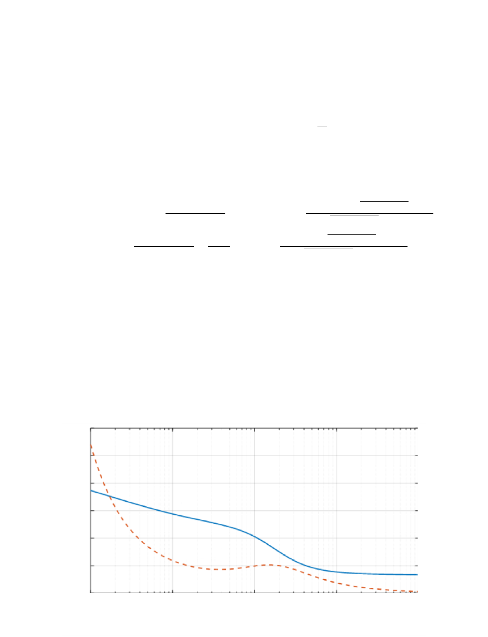
Figure 1 depicts typical values of penetration depth as a function of frequency for different types of
Earth’s surface components including pure water, sea water, dry soil, wet soil, and dry ice. The
penetration depths for pure water and sea water are calculated at 20
o
C, and the salinity of sea water
is 35 g/kg. The penetration depths for dry soil and wet soil assume the volumetric water content is
0.07 and 0.5, respectively. Other soil parameters are the same as in Fig. 7. The penetration depth of
dry ice is calculated at 0
o
C.
Rec. ITU-R P.527-4 5
FIGURE 1
Penetration depth of surface types as a function of frequency
P.05 7-02 1
0.01 0.1 1 10 100 1 000
0.001
0 0. 1
0.1
1
10
1 00
1 00 0
Penetration depth (m)
Frequency GHz ( )
Pure water
Sea water
Dry soil
Wet soil
Dry ice
4 Factors determining the effective electrical characteristics of soil
The effective values of the electrical characteristics of the soil are determined by the nature of the
soil, its moisture content, temperature, general geological structure, and the frequency of the incident
electromagnetic radiation.
4.1 Nature of the soil
Although it has been established by numerous measurements that values of the electrical
characteristics of soil vary with the nature of the soil, this variation may be due to its ability to absorb
and retain moisture rather than the chemical composition of the soil. It has been shown that loam,
which normally has a conductivity on the order of 10
−2
S/m can, when dried, have a conductivity as
low as 10
−4
S/m, which is the same order as granite.
4.2 Moisture content
The moisture content of the ground is the major factor determining the permittivity and conductivity
of the soil. Laboratory measurements have shown that as the moisture content of the ground increases
from a low value, the permittivity and conductivity of the ground increase and reach their maximum
values as the moisture content approaches the values normally found in such soils. At depths of one
metre or more, the wetness of the soil at a particular site is typically constant. Although the wetness
may increase during periods of rain, the wetness returns to its typical value after the rain has stopped
due to drainage and surface evaporation.
The typical moisture content of a particular soil may vary considerably from one site to another due
to differences in the general geological structure which provides different drainage.

6 Rec. ITU-R P.527-4
4.3 Temperature
Laboratory measurements of the electrical characteristics of soil have shown that, at low frequencies
conductivity increases by approximately 3% per degree Celsius, while permittivity is approximately
constant over temperature. At the freezing point, there is generally a large decrease in both
conductivity and permittivity.
4.4 Seasonal variation
The effects of seasonal variation on the electrical characteristics of the soil surface are due mainly to
changes in water content and temperature of the top layer of the soil.
5 Complex relative permittivity prediction methods
The models described in the following sub-sections provide prediction methods for the complex
relative permittivity of the following Earth’s surfaces:
– Pure Water
– Sea (i.e. Saline) Water
– Ice
– Dry Soil (combination of sand, clay, and silt)
– Wet Soil (dry soil plus water)
– Vegetation (above and below freezing)
In this section, subscripts of the complex relative permittivity and hence the subscripts of its real and
imaginary parts are chosen to denote the relative permittivity specialised for specific cases; e.g. the
subscript “pw” for pure water, the subscript “sw” for sea water, etc.
5.1 Water
This sub-section provides prediction methods for the complex relative permittivity of pure water, sea
water, and ice.
5.1.1 Pure water
The complex relative permittivity of pure water,
, is a function of frequency,
, and
temperature, (
o
C):
(5)
(6)
(7)
where:
(8)
(9)
(10)
(11)
and
and
are the Debye relaxation frequencies:
(12)

Rec. ITU-R P.527-4 7
(13)
5.1.2 Sea water
The complex relative permittivity of sea (saline) water,
, is a function of frequency,
(GHz),
temperature, (
o
C), and salinity (g/kg or ppt)
2
.
(14)
(15)
(16)
where
(17)
(18)
(19)
(20)
(21)
Values of
,
,
,
and
are obtained from equations (8), (9), (10), (12), and (13). Furthermore,
is given by
(22)
(23)
(24)
(25)
(26)
(27)
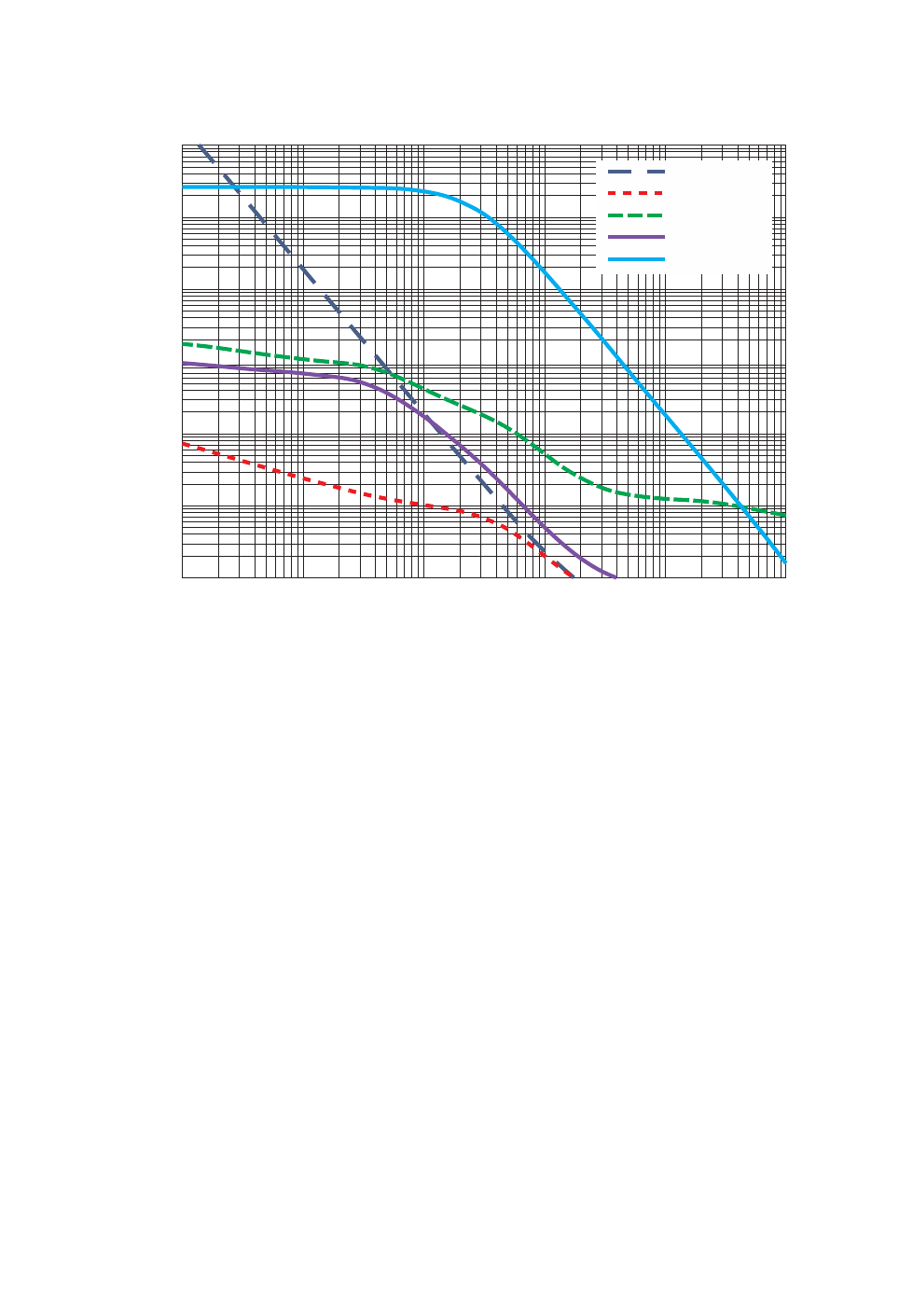
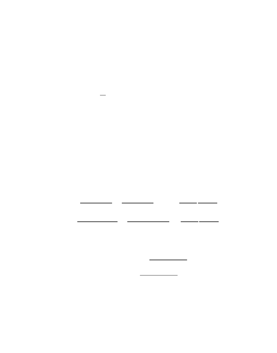
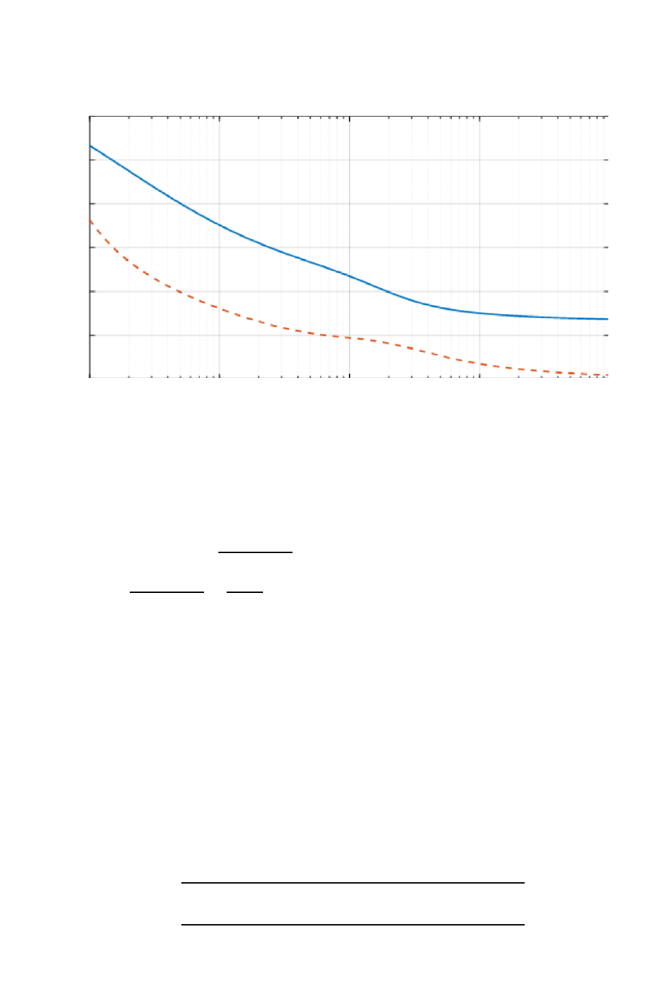
The complex relative permittivity of pure water given in equations (5) – (7) is a special case of
equation (14) – (16) where S = 0. The complex relative permittivity of pure water (S = 0 g/kg) and
sea water (S = 35 g/kg) vs. frequency are shown in Fig. 2 for
o
C and in Figure 3 for
o
C.
2
The term “ppt” stands for “parts per thousand”.
8 Rec. ITU-R P.527-4
FIGURE 2
Complex relative permittivity of pure and sea water as a function of frequency
(
o
C)
P.05 7-022
S = 0.0 g/kg
Complex relative permittivity of water
Frequency GHz ( )
S = 35 g/kg
10
–1
0
100
Real part
Imaginary part
10 10
1
10
2
10
3
100
10
90
80
70
10060
50
40
30
20
FIGURE 3
Complex relative permittivity of pure and sea water as a function of frequency
(
o
C)
P.05 7-032
S = 0.0 g/kg
Complex relative permittivity of water
Frequency GHz ( )
S = 35 g/kg
10
–1
0
100
Real part
Imaginary part
10 10
1
10
2
10
3
100
10
90
80
70
10060
50
40
30
20
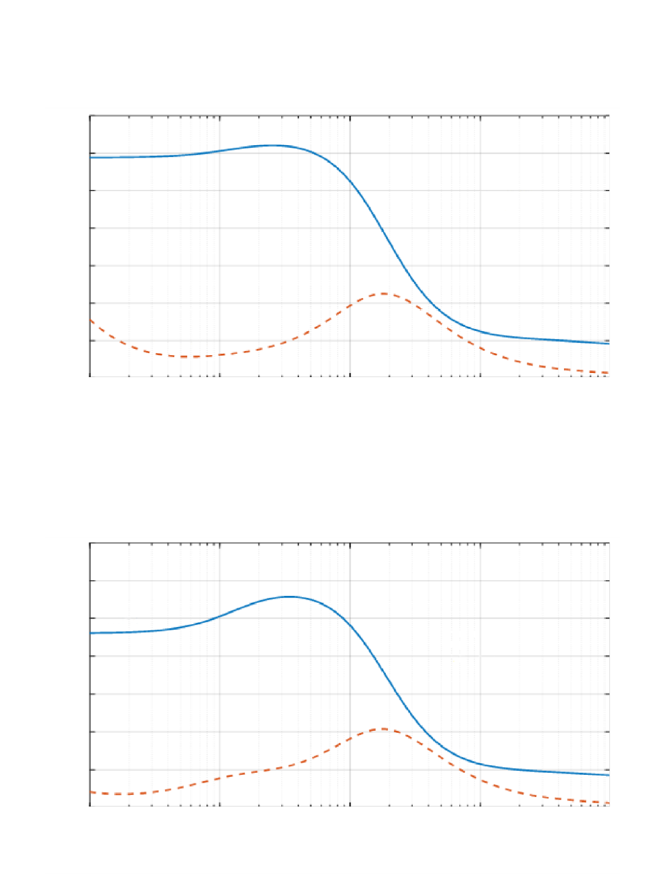
5.1.3 Ice
This sub-section provides prediction methods for the complex relative permittivity of dry ice and wet
ice.

Rec. ITU-R P.527-4 9
5.1.3.1 Dry ice
Dry ice is composed of frozen pure water (i.e. ≤ 0
o
C). The complex relative permittivity of dry
ice,
, is
(28)
The real part of the complex relative permittivity,
, is a function of temperature, (
o
C), and is
independent of frequency:
(29)
and the imaginary part of the complex relative permittivity,
, is a function of temperature (
o
C)
and frequency,
(GHz):
(30)
where
(31)
(32)
(33)
(34)
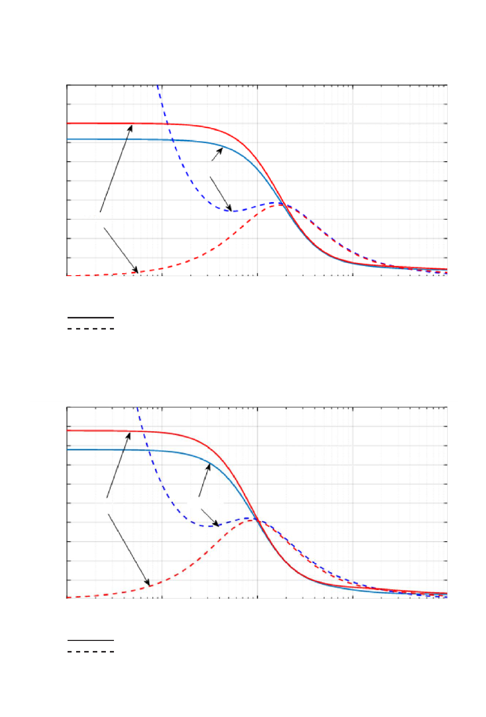
The real and imaginary parts of complex relative permittivity of dry ice are shown in Fig. 4 for
o
C.
5.1.3.2 Wet ice
When the ice is wet (at 0
o
C), its grains are surrounded by liquid water. Considering ice grains as
spherical inclusions within a liquid water background, the Maxwell Garnett dielectric mixing formula
is applied to express the complex relative permittivity of wet ice,
, as a combination of the
complex relative permittivity of dry ice,
, and the complex relative permittivity of pure water,
(35)
is the liquid water volume fraction
. Equation (35) is complex, and it can be split into
the real part and the imaginary part. Each part is a function of the real and imaginary parts of the
complex relative permittivity of dry ice and corresponding parts of water. The real and imaginary
parts of wet ice at
and
o
C are depicted in Fig. 5 as a function of liquid water
content.
10 Rec. ITU-R P.527-4
FIGURE 4
Complex relative permittivity of dry ice as a function of frequency
(
o
C)
P.05 7-042
Complex relative permittivity of dry ice
Frequency GHz ( )
10
–1
Real part
Imaginary part
10 10
1
10
2
10
3
10
–4
10
–3
10
–2
10
–1
10
10
1
FIGURE 5
Complex relative permittivity of wet ice as a function of liquid water content
( and
o
C)
P.05 7-052
Complex relative permittivity of wet ice
Liquid water content fractionm /m ( )
3 3
0
Real part
Imaginary part
0
2
4
6
8
10
12
14
0.1 0.2 0.3 0.4 0.5 0.6 0.7 0.8 0.9 1
5.2 Soil
The complex relative permittivity of soil,
, is a function of frequency,
(GHz), temperature,
(
o
C), soil composition, and volumetric water content.
The soil composition is characterized by the percentages by volume of the following dry soil
constituents which are available from field surveys and laboratory analysis: a)
= % sand, b)
= % clay, and c)
= % silt as well as d) the specific gravity
(i.e. the mass density of soil
Rec. ITU-R P.527-4 11
divided by the mass density of water) of the dry mixture of soil constituents,
, and e) the volumetric
water content,
, equal to the water volume divided by total soil volume for a given soil sample.
The bulk density
(i.e. the mass of soil in a given volume (g cm
−3
) of the soil,
, is also required as
an input. While it is not easily measured directly, it can be derived from the percentages of the dry
constituents. If a local pseudo-transfer function is not available, the following empirical
pseudo-transfer function can be used
(36)
Equation (36) is not reliable for less than 1% of any constituent. If the percentages of a constituent
are less than 1%, the corresponding term in equation (36) should be omitted. The constituent
percentages of the included terms should sum to 100%.
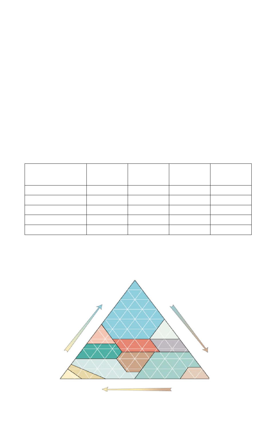
Table 1 shows typical constituent percentages, specific gravities, and bulk densities for four
representative soil types.
TABLE 1
Physical parameters of various soil types
Soil Designation
Textural Class
1
Sandy Loam
2
Loam
3
Silty Loam
4
Silty Clay
% Sand
51.52
41.96
30.63
5.02
% Clay
13.42
8.53
13.48
47.38
% Silt
35.06
49.51
55.89
47.60
2.66
2.70
2.59
2.56
(g cm
−3
)
1.6006
1.5781
1.5750
1.4758
FIGURE 6
Soil texture triangle
P.05 7-062
Clay
100
10
20
30
40
50
60
70
80
90
100
1
0
2
0
3
0
4
0
5
0
6
0
7
0
8
0
9
0
1
0
0
90
10
20
30
40
50
60
70
80
Silty
clay
Silt
Sand
Loamy
sand
Sandy loam
Loam
Clay loam
Sandy clay loam
Sandy
clay
Silty clay
loam
Silt loam
P
e
r
c
e
n
t
s
i
l
t
P
e
r
c
e
n
t
c
l
a
y
The soil designation textural class reported in the first row of Table 1 is based on the soil texture
triangle depicted in Fig. 6.
12 Rec. ITU-R P.527-4
This prediction method considers soil as a mixture of four components: a) soil particles composed of
a combination of clay, sand, and silt, b) air, c) bound water (water attached to soil particles by forces
such as surface tension, where the thickness of the water layer and its dielectric constant and
relaxation frequencies are unknown), and d) free water (also known as bulk water that flows freely
within soil bores). The complex relative permittivity of soil,
, of this four component mixture is
(37)
where:
(38)
(39)
(40)
(41)
(42)
and
α = 0.65 (43)
and
are the real and the imaginary parts of the complex relative permittivity of free water:
(44)
(45)
where
,
,
,
and
are obtained from equations (8), (9), (10), (12), and (13), and
and
are:
(46)
(47)
and
(48)
(49)
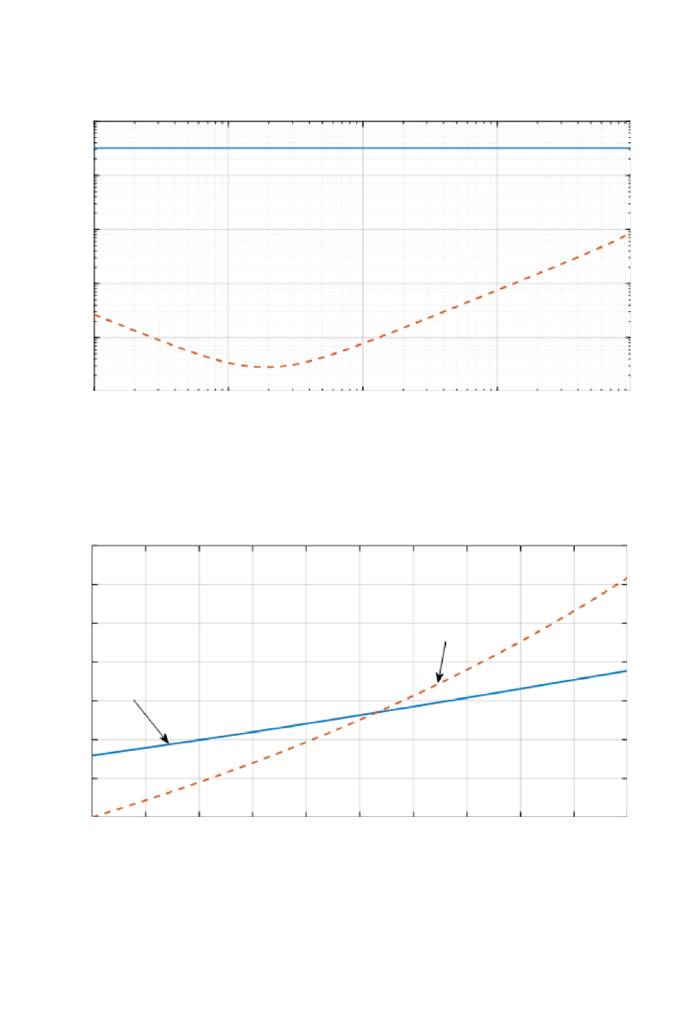
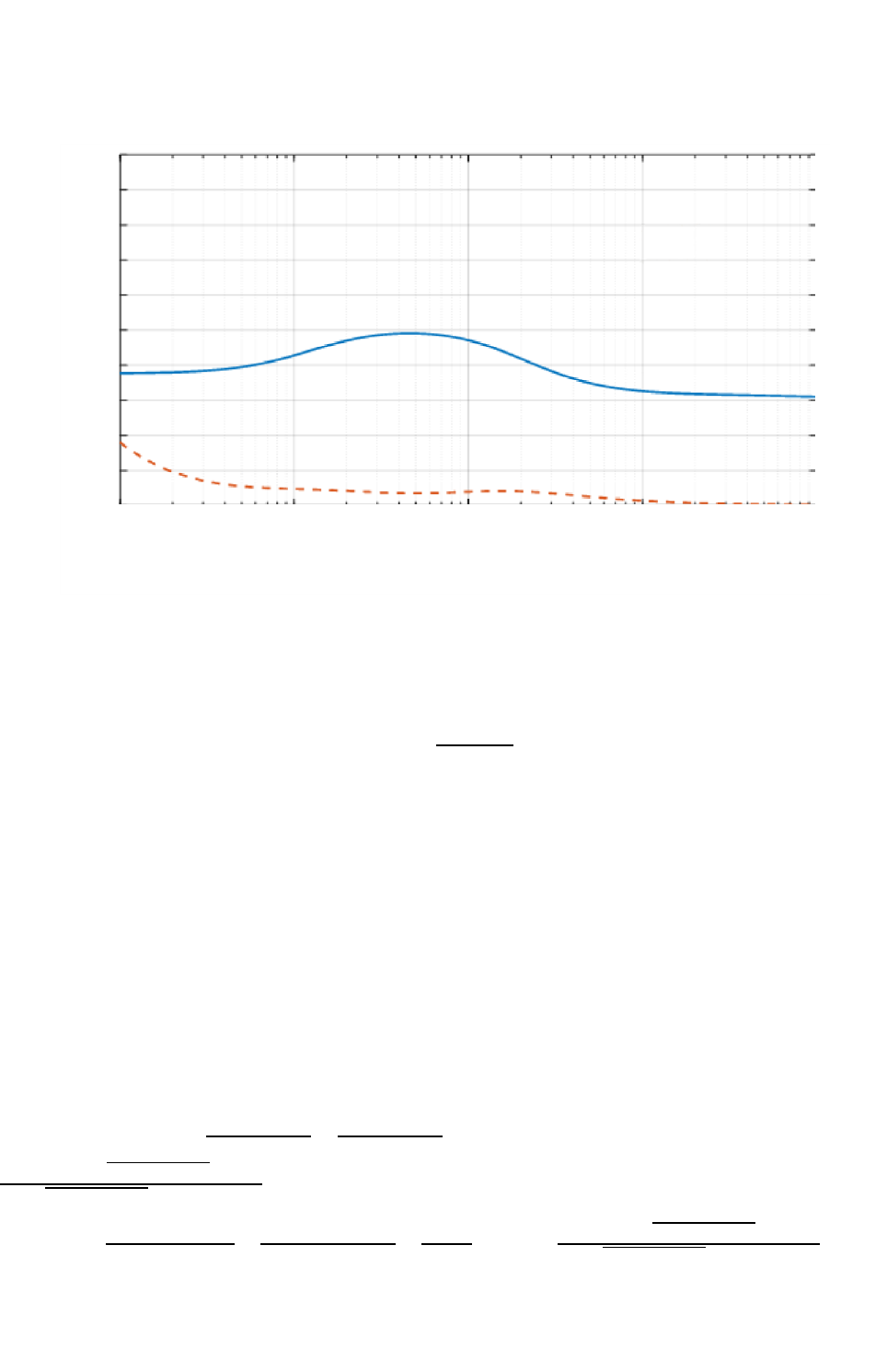
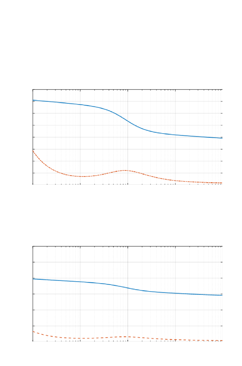
The complex relative permittivity of two examples of soil types are shown in Figs 7, 8 and 9. The soil
composition in Figs 7 and 9 are identical except for the volumetric water content, indicating that both
the real part and imaginary part of the complex relative permittivity are directly related to the
volumetric water content.
Rec. ITU-R P.527-4 13
FIGURE 7
Complex relative permittivity of a silty loam soil as a function of frequency
(
= 0.5, =23
o
C,
)
P.05 7-072
Imaginary part
Complex relative permittivity of soil
Frequency GHz ( )
Real part
10
–1
0
35
Sand: 30.63%
Clay: 13.48%
Silt: 55.86%
10 10
1
10
2
10
3
10
30
20
5
15
25
FIGURE 8
Complex relative permittivity of a silty clay soil as a function of frequency
(
= 0.5, =23
o
C,
)
P.05 7-082
Sand:5.02%
Clay:47.38%
Silt: 47.60%
Imaginary part
Complex relative permittivity of soil
Frequency GHz ( )
Real part
10
–1
0
35
10 10
1
10
2
10
3
10
30
20
5
15
25
14 Rec. ITU-R P.527-4
FIGURE 9
Complex relative permittivity of a silty loam soil as a function of frequency
(
= 0.07, =23
o
C,
)
P.05 7-092
Sand:30.63%
Clay:13.48%
Silt: 55.89%
Imaginary part
Complex relative permittivity of soil
Frequency GHz ( )
Real part
10
–1
0
10
10 10
1
10
2
10
3
3
5
4
1
2
7
9
8
6
5.3 Vegetation
The complex relative permittivity of vegetation is a function of frequency
(GHz), temperature
(
o
C), and vegetation gravimetric water content,
, which is defined as
(50)
is the weight of the moist vegetation, and
is the weight of the dry vegetation.
is between
0.0 and 0.7.
This prediction method considers the vegetation as a mixture of bulk vegetation, saline free water,
bounded water, and ice (if applicable). The complex relative permittivity of this mixture is given by
(51)
The real part,
, and the imaginary part,
, of the complex relative permittivity of vegetation are
given in § 5.3.1 for above freezing temperatures, and in § 5.3.2 for below freezing temperatures.
5.3.1 Above freezing temperatures
At temperatures above freezing ( > 0 C), the real, and imaginary parts of the complex relative
permittivity of vegetation are:
(52)
(53)
where
is the real part of the relative permittivity of bulk vegetation,
is the free water volume
fraction, and
is the bound water volume fraction with:
(54)
Rec. ITU-R P.527-4 15
(55)
(56)
is the electrical conductivity of saline water given in equations (22) to (27), where the salinity,
, is
(57)
and
,
,
,
and
are obtained from equations (8), (9), (10), (12) and (13) respectively.
For a temperature of 22 °C and a frequency range up to 40 GHz, equations (52) and (53) are modified
as follows:
(58)
(59)
Equations (58) and (59) are more general than equation (16) of Recommendation ITU-R P.833 since
they account for both free and bound water and include the temperature dependence.
The real and imaginary parts of the complex relative permittivity of vegetation vs. frequency at two
different values of gravimetric water content are shown in Figs 10 and 11 demonstrating that both the
real part and the imaginary part of the complex relative permittivity of vegetation increase as the
gravimetric water content increases.
FIGURE 10
Complex relative permittivity of vegetation as a function of frequency
(
o
C)
P.05 7-102
Imaginary part
Complex relative permittivity of vegetation
Frequency z ( )GH
Real part
10
–1
0
10 10
1
10
2
10
3
10
20
30
40
50
60
16 Rec. ITU-R P.527-4
FIGURE 11
Complex relative permittivity of vegetation as a function of frequency
(
o
C)
P.05 7-112
Imaginary part
Complex relative permittivity of vegetation
Frequency GHz ( )
Real part
10
–1
0
10 10
1
10
2
10
3
2
4
6
8
10
12
5.3.2 Below freezing temperatures
For below freezing temperatures between (−20 C ≤ < 0 C) the real and imaginary parts of the
complex relative permittivity are:
(60)
(61)
where:
(62)
(63)
(64)
(65)
(66)
(67)
(68)
(69)
(70)
(71)
and the vegetation freezing temperature,
, is −6.5
o
C.
Rec. ITU-R P.527-4 17
The real and the imaginary parts of the complex relative permittivity vs. frequency and temperature
are shown in Figs 12 and 13. These Figures show that reducing the temperature below freezing
decreases both the real and imaginary parts of the vegetation complex relative permittivity, and
decreases the dependence of those parameters on frequency. For frequencies above 20 GHz, the
complex relative permittivity of vegetation becomes less dependent on temperature.
FIGURE 12
Complex relative permittivity of vegetation as a function of frequency
(
o
C)
P.05 7-122
Imaginary part
Complex relative permittivity of vegetation
Frequency GHz ( )
Real part
10
–1
0
10 10
1
10
2
10
3
2
4
6
8
10
12
14
16
FIGURE 13
Complex relative permittivity of vegetation as a function of frequency
(
o
C)
P.05 7-132
Imaginary part
Complex relative permittivity of vegetation
Frequency GHz ( )
Real part
10
–1
0
10 10
1
10
2
10
3
2
4
6
8
10
12

18 Rec. ITU-R P.527-4
Appendix
to Annex 1
Electrical properties expressed as permittivity and conductivity
as used in Recommendations ITU-R P.368 and ITU-R P.832
1 Introduction
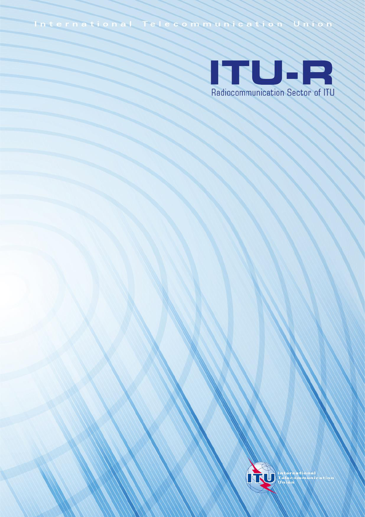
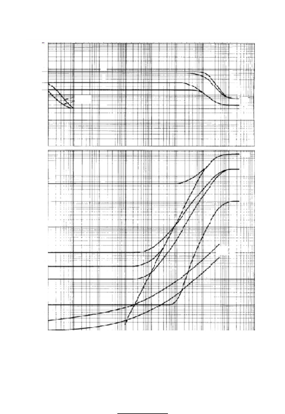
Figure 14 below is reproduced from Fig. 1 showing typical values of conductivity and permittivity
for different types of ground, as a function of frequency. These graphs are retained from earlier
revisions of this Recommendation as a convenience to users of Recommendation ITU-R P.386 and
ITU-R P.832.
Rec. ITU-R P.527-4 19
FIGURE 14
Relative permittivity ε
r
, and conductivity σ, as a function of frequency
P.05 7-142
Conductivity, (S/m)
Frequency MHz ( )
C,F
80
10
2
A
B
D
E,G
A
B
C
D
E
F
A,C,F
B,D
E
A,C,F
B,D
E
– 1°C
G
– 10°C
A: Sea water (average salinity), 20° C
B: Wet ground
C: Fresh water, 20° C
D: Medium dry ground
E: Very dry ground
F: Pure water, 20° C
G: Ice (fresh water)
– 1°C
G
– 10°C
2
5
30
15
2
5
10
2
5
1
2
5
10
3
2
5
10
2
10
–1
10
2
5
1
10
–1
2
5
2
5
2
5
10
–3
2
5
2
5
10
–2
10
–5
10
–4
10
–2
52
10
–1
52
10
52
10
2
52
10
3
52
10
4
52
10
5
52
10
6
1
52
