
International Telecommunication Union
Recommendations
Radiocommunication Sector
Recommendation ITU-R P.2040-3
(08/2023)
P Series: Radiowave propagation
Effects of building materials and
structures on radiowave propagation
above about 100 MHz

ii Rec. ITU-R P.2040-3
Foreword
The role of the Radiocommunication Sector is to ensure the rational, equitable, efficient and economical use of the radio-
frequency spectrum by all radiocommunication services, including satellite services, and carry out studies without limit
of frequency range on the basis of which Recommendations are adopted.
The regulatory and policy functions of the Radiocommunication Sector are performed by World and Regional
Radiocommunication Conferences and Radiocommunication Assemblies supported by Study Groups.
Policy on Intellectual Property Right (IPR)
ITU-R policy on IPR is described in the Common Patent Policy for ITU-T/ITU-R/ISO/IEC referenced in Resolution
ITU-R 1. Forms to be used for the submission of patent statements and licensing declarations by patent holders are
available from http://www.itu.int/ITU-R/go/patents/en where the Guidelines for Implementation of the Common Patent
Policy for ITU-T/ITU-R/ISO/IEC and the ITU-R patent information database can also be found.
Series of ITU-R Recommendations
(Also available online at https://www.itu.int/publ/R-REC/en)
Series
Title
BO
Satellite delivery
BR
Recording for production, archival and play-out; film for television
BS
Broadcasting service (sound)
BT
Broadcasting service (television)
F
Fixed service
M
Mobile, radiodetermination, amateur and related satellite services
P
Radiowave propagation
RA
Radio astronomy
RS
Remote sensing systems
S
Fixed-satellite service
SA
Space applications and meteorology
SF
Frequency sharing and coordination between fixed-satellite and fixed service systems
SM
Spectrum management
SNG
Satellite news gathering
TF
Time signals and frequency standards emissions
V
Vocabulary and related subjects
Note: This ITU-R Recommendation was approved in English under the procedure detailed in Resolution ITU-R 1.
Electronic Publication
Geneva, 2023
© ITU 2023
All rights reserved. No part of this publication may be reproduced, by any means whatsoever, without written permission of ITU.
Rec. ITU-R P.2040-3 1
RECOMMENDATION ITU-R P.2040-3
Effects of building materials and structures on radiowave
propagation above about 100 MHz
(Question ITU-R 211/3)
(2013-2015-2021-2023)
Scope
This Recommendation provides guidance on the effects of building materials and structures on radio-wave
propagation above 100 MHz.
Keywords
Permittivity, conductivity
The ITU Radiocommunication Assembly,
considering
a) that electrical properties of materials and their structures strongly affect radiowave propagation;
b) that it is necessary to understand the losses of radiowaves caused by building materials and
structures;
c) that there is a need to give guidance to engineers to avoid interference from outdoor to indoor
and indoor to outdoor systems;
d) that there is a need to provide users with a unified source for computing effects of building
materials and structures,
noting
a) that Recommendation ITU-R P.526 provides guidance on diffraction effects, including those
due to building materials and structures;
b) that Recommendation ITU-R P.527 provides information on the electrical properties of the
surface of the Earth;
c) that Recommendation ITU-R P.679 provides guidance on planning broadcasting-satellite systems;
d) that Recommendation ITU-R P.1238 provides guidance on indoor propagation over the
frequency range 900 MHz to 100 GHz;
e) that Recommendation ITU-R P.1406 provides information on various aspects of propagation
relating to terrestrial land mobile and broadcasting services in the VHF and UHF bands;
f) that Recommendation ITU-R P.1407 provides information on various aspects of multi-path
propagation;
g) that Recommendation ITU-R P.1411 provides propagation methods for short paths in
outdoor situations, in the frequency range from about 300 MHz to 100 GHz;
h) that Recommendation ITU-R P.1812 provides a propagation prediction method for terrestrial
point-to-area services in the frequency range 30 MHz to 6 GHz,
2 Rec. ITU-R P.2040-3
recommends
that the information and methods in Annex 1 should be used as a guide for the assessment of the
effects of building material properties and structures on radiowave propagation, and in developing
deterministic models of propagation involving the built environment.
Annex 1 describes basic principles, and provides expressions to evaluate reflection from and
transmission through building materials and structures. It also includes a model for electrical
properties as a function of frequency, and a table of parameters for relevant materials.
Examples of building-entry loss measurements may be found in Report ITU-R P.2346.
Annex 1
TABLE OF CONTENTS
Page
Policy on Intellectual Property Right (IPR) ............................................................................. ii
Annex 1 .................................................................................................................................... 2
1 Introduction .................................................................................................................... 3
2 Basic principles and theory ............................................................................................. 3
2.1 Theory of material electrical properties .............................................................. 3
2.1.1 Introduction .......................................................................................... 3
2.1.2 Method ................................................................................................. 3
2.1.3 Frequency dependence of material properties...................................... 7
2.1.4 Models of material properties frequency dependence ......................... 8
2.2 Effects of material structure on radiowave propagation ..................................... 8
2.2.1 Plane wave reflection and transmission at a single planar interface .... 8
2.2.2 Plane wave reflection and transmission for a single- or multi-layer
slab ....................................................................................................... 12
2.2.3 Waveguide propagation in buildings ................................................... 16
2.3 Theory and results for frequency selective surface materials ............................. 19
2.3.1 Frequency selective surfaces ................................................................ 19
2.3.2 Theory for wave propagation around the surface of round convexity
array...................................................................................................... 20
2.3.3 Calculation results ................................................................................ 21
2.3.4 Measurement ........................................................................................ 22
Rec. ITU-R P.2040-3 3
3 Compilations of electrical properties of materials .......................................................... 23
Attachment 1 to Annex 1 Alternative method to obtain reflection and transmission
coefficients for building materials represented by N dielectric slabs based on ABCD
matrix formulation .......................................................................................................... 25
1 Introduction
This Annex provides guidance on the effects of building material electrical properties and structures
on radio-wave propagation.
Section 2 describes fundamental principles concerning the interaction of radio waves with building
materials, defines various parameters in use for these purposes, and gives basic expressions for
reflection from and transmission through single material interfaces and single and multiple layer
slabs, typical of building construction.
Section 3 defines a model for electrical properties, and a table of parameters for various building
materials.
2 Basic principles and theory
Radio waves that interact with a building will produce losses that depend on the electrical properties
of the building materials and material structure. In this section, theoretical effects of material
electrical properties and structure on radio-wave propagation will be discussed.
2.1 Theory of material electrical properties
2.1.1 Introduction
This section describes the development of simple frequency-dependent formulae for the permittivity
and conductivity of common building materials. The formulae are based on curve fitting to a number
of published measurement results, mainly in the frequency range 1-100 GHz. The aim is to find a
simple parameterization for use in indoor-outdoor ray trace modelling.
The characterization of the electrical properties of materials is presented in a number of different
ways in the literature. These are described in § 2.1.2 in order that the measured data can be reduced
to a common format.
2.1.2 Method
2.1.2.1 Definitions of electrical constants
The following treatment deals only with non-ionized, non-magnetic materials, and throughout we
therefore set the free charge density,
f
, to zero and the permeability of the material, , to the
permeability of free space
0
.
The fundamental quantities of interest are the electrical permittivity, , and the conductivity, . There
are many ways of quantifying these parameters in the literature, so we first make explicit these
different representations and the relations between them.
2.1.2.2 Derivation
The starting point is the wave equation derived from Maxwell’s equations. Under the above
assumptions, the wave equation for the electric field is:
E

4 Rec. ITU-R P.2040-3
t
J
t
E
E
f
=
0
2
2
0
2
–
(1)
where:
: (vector) electric field intensity (V/m)
J
f
: current density of free charges (A/m
2
)
: dielectric permittivity (F/m)
0
: permeability of free space (N/A
2
) = 4 10
−
7
by definition.
In a conductor, is related to through Ohm’s Law by:
EJ
f
=
(2)
where:
: conductivity (S/m).
Combining equations (1) and (2) gives:
t
E
t
E
E
=
0
2
2
0
2
–
(3)
Writing in exponential notation:
( )
rktj
eEE
=
–
0
(4)
where:
: value of for t = = 0 (V/m)
: (vector) wave number (m
−1
) magnitude = 2/ where is the wavelength in m
: angular frequency (s
−
1
) = 2f where f is the frequency in s
−
1
: (vector) spatial distance (m).
and substituting in equation (3) gives:
0–
0
2
0
2
=+ jk
(5)
where:
k : magnitude of .
Equation (5) shows that the electric field intensity propagates as an attenuated sinusoidal wave.
E
f
J
E
E
0
E
E
r
k
k
Rec. ITU-R P.2040-3 5
2.1.2.3 Non-conducting dielectric
In a non-conducting dielectric ( = 0) the field is unattenuated and from equation (5) the velocity of
propagation, v (= /k), is:
(6)
is conventionally written in terms of the relative permittivity and the permittivity of free space:
(7)
where:
: relative dielectric permittivity of the medium concerned
0
: dielectric permittivity of free space = 8.854 10
−12
(F/m).
Thus the velocity of propagation in a medium of relative permittivity can be written:
(8)
where c is the velocity of light in free space (= ). In other words,
is the refractive index
of the dielectric medium.
2.1.2.4 Conducting dielectric
When 0, the wave attenuates as it propagates. It is convenient in this case to define a complex
relative permittivity which may be derived as follows. Equation (5) can be rearranged, with the
substitution
( )
00
2
/1 =c
, to give:
(9a)
Since equation (8) gives
=
2
2
c
, this can be interpreted as a complex relative permittivity given by:
−=
0
' j
(9b)
This shows that the relative permittivity defined for a pure dielectric, becomes the real part ' of the
more general, complex relative permittivity defined for a conducting dielectric.
There are no universally accepted symbols for these terms. In this Recommendation, relative
permittivity is written in the form:
−
= j
(10)
where ' and '' are the real and imaginary parts. Using equation (9b), the imaginary part is given by:
=
0
(11)
Note that the sign of the imaginary part of is arbitrary, and reflects the sign convention in
equation (4). In practical units, equation (11) gives a conversion from " to :
GHz
05563.0 f
=
(12)
Another formulation of the imaginary part of is in terms of the loss tangent, defined as:
0
1
=v
00
/1
6 Rec. ITU-R P.2040-3
(13)
and so:
(14)
From equation (10) this gives:
(15)
and in practical units:
(16)
Another term sometimes encountered is the Q of the medium. This is defined as:
(17)
and is the ratio of the displacement current density to the conduction current density J
f
. For
non-conductors, Q → . From equation (14):
(18)
Yet another term encountered is the complex refractive index n which is defined to be
. Writing
n in terms of its real and imaginary parts:
=
−
= njnn
(19)
', " and are given from equations (10) and (12) by:
GHz
1113.0
2
2
)(–
2
)(
fnn
nn
nn
=
=
=
(20)
2.1.2.5 Attenuation rate
A conducting dielectric will attenuate electromagnetic waves as they propagate. To quantify this,
substitute equation (5) in equation (4) and simplify using equation (14):
( )
( )
rkjtjEE
=
00
tan–1'–exp
(21)
where:
: (vector) wave number (m
−
1
) in free space.
The imaginary part under the square root sign leads to an exponential decrease of the electric field
with distance:
(22)
In a practical calculation using complex variables, the attenuation distance, , at which the field
amplitude falls by 1/e, can be evaluated as:
tD /
0
k
Rec. ITU-R P.2040-3 7
( )
−
=
0
Im
1
k
(23a)
where the function “Im” returns the imaginary part of its argument. Analytically it can be shown that:
( )
−
=
cos1
cos2
'
1
0
k
(23b)
which can be evaluated by calculating tan from
'
and and inverting to obtain cos . More direct
evaluation is possible in the two limits of → 0 (dielectric limit) and → (good conductor limit).
By choosing the appropriate approximation of the term under the square root sign in equation (21)
these limits are:
=
tan
2
'
1
0
k
dielectric
(24)
and:
=
tan
2
'
1
0
k
conductor
(25)
Equations (24) and (25) are accurate to about 3% for tan < 0.5 (dielectric) tan > 15 (conductor).
conductor
is usually referred to as the “skin depth”.
For practical purposes the attenuation rate is a more useful quantity than the attenuation distance, and
is related to it simply by
(26)
where:
A: attenuation rate in dB/m (with in m).
Substituting equations (24) and (25) in equation (26) and converting to practical units gives:
=1636
dielectric
A
(27a)
GHz
8.545 fA
conductor
=
(27b)
2.1.3 Frequency dependence of material properties
In the literature, the real part of the dielectric constant, ', is always given, but often the frequency is
not specified. In practice for many materials, the value of ' is constant from DC up to around
5-10 GHz after which it begins to fall with frequency.
The value of is usually a strong function of frequency in the band of interest, increasing with
frequency. This may be one reason why the imaginary part of the dielectric constant, or the loss
tangent, is often specified in the literature: equations (12) and (16) show that these terms remove a
linear frequency dependence compared to the frequency dependence of .
=
= /686.8
log20
10
e
A
8 Rec. ITU-R P.2040-3
For each material a simple regression model for the frequency dependence of can be obtained by
fitting to measured values of at a number of frequencies.
2.1.4 Models of material properties frequency dependence
In order to derive the frequency dependence of material properties, the values of the electrical
constants of the materials can be characterized in terms of the measurement frequency, real part (')
and imaginary part ('') of the relative permittivity, loss tangent (tan ) and conductivity ().
Expressions in § 2.1.2.4 permit conversions between these quantities.
For the conductivity, there is usually statistically significant evidence for an increase with frequency.
In this case the trend has been modelled using:
d
fc
GHz
=
(28)
where c and d are constants characterizing the material. This is a straight line on a log()–log(f) graph.
The trend line is the best fit to all available data.
For the relative permittivity one can assume similar frequency dependency:
b
fa
GHz
=
(29)
where a and b are constants characterizing the material. However, in almost all cases there is no
evidence of a trend of relative permittivity with frequency. In these cases, a constant value can be
used at all frequencies. The constant value is the mean of all the values plotted. Some examples are
given in Table 3.
2.2 Effects of material structure on radiowave propagation
2.2.1 Plane wave reflection and transmission at a single planar interface
This section considers a plane wave incident upon a planar interface between two homogeneous and
isotropic media of differing electric properties. The media extend sufficiently far from the interface
such that the effect of any other interface is negligible. This may not be the case with typical building
geometries. For example, propagation losses due to a wall may be influenced by multiple internal
reflections. Methods for calculating reflection and transmission coefficients of single-layer and multi-
layer slabs are given in § 2.2.2.
A plane wave is useful for analysis purposes, but the concept is largely theoretical. In practice a wave
may approximate but not be exactly planar. The point is important here because a truly plane wave
does not experience free-space (spreading) loss. The following methods take no account of free-space
losses, only the effect of the media interface.
2.2.1.1 Oblique incidence on a plane media interface
Figure 1 illustrates a sinusoidal plane wave incident obliquely to a plane interface separating two
uniform non-magnetic dielectric media having relative permittivities
1
and
2
. Values for can be
calculated from the real part of the permittivity, ', and conductivity, , using equations (10) and (11).
Table 3 provides parameters from which these can be calculated as functions of frequency.
There are three important theorems for this case that follow from geometrical considerations.
1) The vector wave numbers of the reflected and transmitted (refracted) waves lie in the plane
of incidence, i.e. the plane defined by wave number k
i
of the incident wave and the normal
to the interface. This is taken to be the x-z plane in Fig. 1.
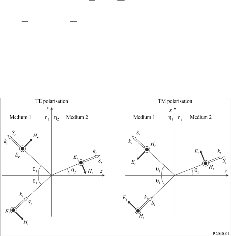
Rec. ITU-R P.2040-3 9
2) The angles of incidence and reflection are equal (both
in Fig. 1).
3) The angle of refraction,
is related to the angle of incidence by Snell’s law.
2
2
1
1
sin
1
sin
1
=
cc
(30)
where
and
are the respective wave speeds in the two media, and
1
and
2
represent the complex relative permittivities of the two media.
These theorems ensure that the exponential space-time factors,
( )
exp –j t k r
, for the three waves
(
2
´
11
,, kkkk →
, respectively) are identical at all points in the interface.
FIGURE 1
Reflection and refraction of plane waves at plane interface
Two polarizations of the incident wave are shown in Fig. 1.
a) On the left the incident electric vector E
i
is perpendicular to the plane of incidence.
This is known as transverse electric (TE) polarisation. Other terms are perpendicular
polarisation, s-polarisation, and -polarisation.
b) On the right the incident electric vector E
i
is parallel to the plane of incidence.
This is known as transverse magnetic (TM) polarisation. Other terms are parallel polarisation,
p-polarization, and -polarization.
In the following descriptions, polarization will be designated by TE or TM.
An arbitrarily or circularly polarised wave can be resolved into its TE and TM components for
calculation purposes, which can then be re-combined.
E-field reflection and transmission coefficients are defined as the ratios of reflected and transmitted
(refracted) vectors respectively to the corresponding incident vector as they exist at the interface. In
general such coefficients are complex. The following expressions take no account of free-space or
other losses prior or subsequent to the interaction of a wave with the interface.
10 Rec. ITU-R P.2040-3
The requirement that electric and magnetic vectors are continuous in the plane of the interface give
the following expressions for electric field coefficients. Reflection and transmission coefficients are
denoted by R and T respectively. The subscripts indicate the vectors concerned, and whether the
polarization is TE or TM. Each of equations (31a) to (32b) are in two parts, according to whether
total internal reflection occurs. Total internal reflection is only possible when a wave is incident upon
a medium with lower refractive index.
E-field reflection coefficient for TE polarisation:
+
−
==
1sin1
1sin
coscos
coscos
1
2
1
1
2
1
2211
2211
i
r
eTE
E
E
R
(31a)
E-field reflection coefficient for TM polarisation:
+
−
==
1sin1
1sin
coscos
coscos
1
2
1
1
2
1
2112
2112
i
r
eTM
E
E
R
(31b)
E-field transmission coefficient for TE polarisation:
+
==
1sin0
1sin
coscos
cos2
1
2
1
1
2
1
2211
11
i
t
eTE
E
E
T
(32a)
E-field transmission coefficient for TM polarisation:
+
==
1sin0
1sin
coscos
cos2
1
2
1
1
2
1
2112
11
i
t
eTM
E
E
T
(32b)
where
1
and
2
are the complex relative permittivities of medium 1 and 2 respectively. These can
be evaluated using equation (9b) with values of ' and obtained from § 3 and Table 3.
The cos
2
terms in equations (31a) to (32b) can be evaluated in terms of
1
using equation (30) as:
1
2
sin
2
1
1
2
cos
−=
(33)
At
1
= 0 the incidence plane is not uniquely defined. In this case all directions of propagation are
normal to the interface, and the coefficient amplitudes from the expression for each polarisation is
the same. In the case of reflection there is an apparent sign change. This arises purely from how the
polarizations are defined; it is not a physical discontinuity.
Rec. ITU-R P.2040-3 11
2.2.1.2 Calculation examples
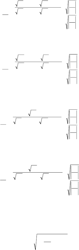
Figure 2 gives examples of reflection and transmission coefficient amplitudes for a wave in air
incident upon concrete at 1 GHz calculated over a range of incidence angles for both polarizations
using equations (31a) to (32b), taking the properties of concrete from Table 3.
FIGURE 2
Reflection and transmission coefficients for air/concrete interface at 1 GHz
2.2.1.3 Substitutions available in coefficient values
It can be useful to note the following substitutions for E-vector coefficients, where the subscripts
denote the medium, 1 or 2, in which the wave is incident on an interface:
a) For either polarisation,
21
RR −=
, and thus
2
2
2
1
RR =
b) For either polarisation,
2
21
1 RTT −=
, where according to a) R can be either R
1
or R
2
.
2.2.1.4 Coefficients for power flux-densities
Coefficients for power flux densities can be obtained from the E-vector coefficients:
2
eTE
R
i
S
r
S
sTE
R ==
(34a)
2
eTM
R
i
S
r
S
sTM
R ==
(34b)
1
2
2
==
eTE
i
t
sTE
T
S
S
T
(35a)
1
2
2
==
eTM
i
t
sTM
T
S
S
T
(35b)
The change in signal level in decibels due to reflection or transmission is thus given by
( )
S
Rlog10
or
( )
S
Tlog10
where R
S
and T
S
stand for either reflection or transmission S-vector coefficient in equations
(34a) to (35b).
12 Rec. ITU-R P.2040-3
Conservation of energy at the media interface requires that for a given incident wavefront area,
the sum of the reflected and transmitted power flux equals the incident power flux. To illustrate this,
account must be taken of the change in wavefront width upon refraction. For either polarization:
1
cos
cos
1
2
=
+
SS
TR
(36)
where
1
2
cos
cos
adjusts for the change in wavefront width.
2.2.1.5 Simplified expressions for incident wave in air
When medium 1 is air, equations (31a) to (32b) can be simplified to:
−+
−−
=
2
2
sincos
sincos
eTE
R
(37a)
−+
−−
=
2
2
sincos
sincos
eTM
R
(37b)
−+
=
2
sincos
cos2
eTE
T
(38a)
−+
=
2
sincos
cos2
eTM
T
(38b)
where is the angle of incidence and is the relative permittivity of the medium upon which the
wave is incident.
Total internal reflection at the interface is not possible in equations (37a) to (38b) since it can be
assumed that the wave is incident upon a medium with a higher refractive index than air.
2.2.2 Plane wave reflection and transmission for a single- or multi-layer slab
2.2.2.1 General method for a multi-layer slab
Figure 3 illustrates a plane wave incident upon a slab consisting of N layers, each with smooth, planar
and parallel surfaces, where N can be 1 or more. The relative permittivity of layer n is
n
, and its
width d
n
metres. It is assumed that the slab is in air, and for calculation purposes this is designated as
layers 0 and N + 1, with relative permittivity 1 and width 0.
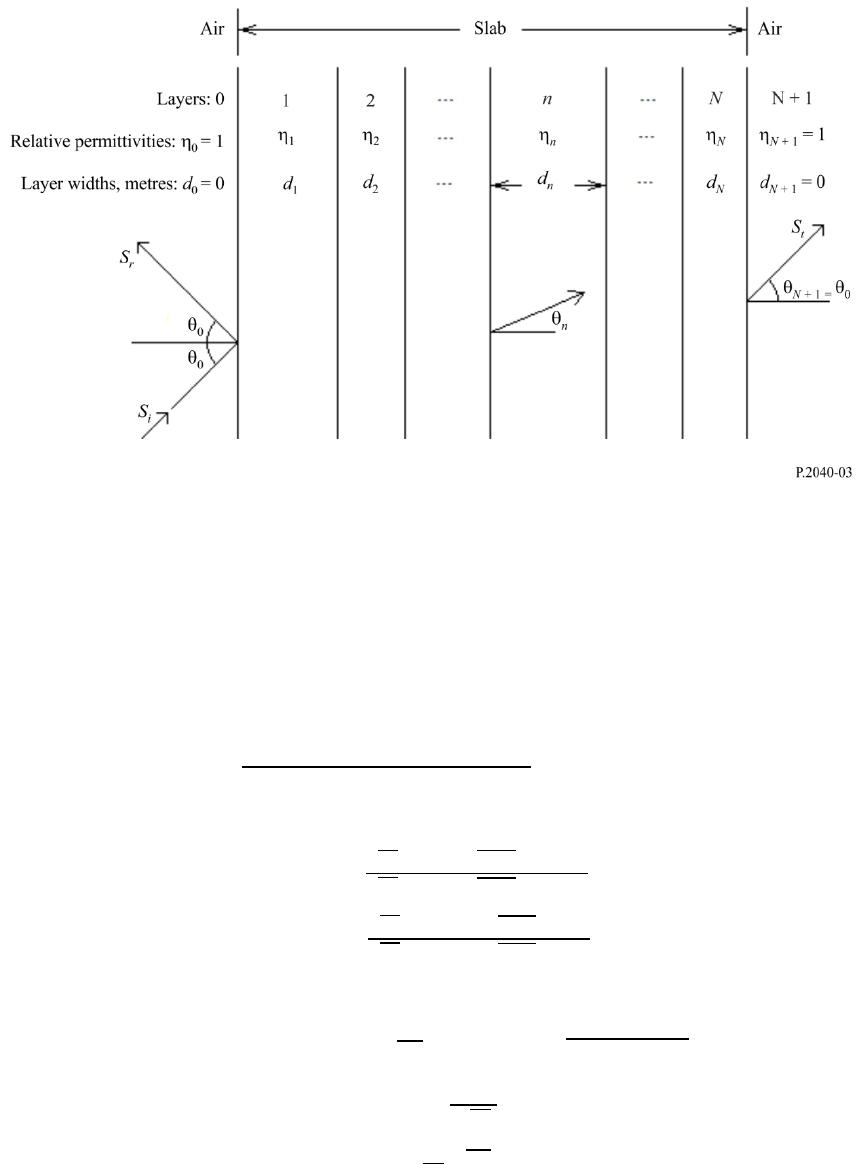
Rec. ITU-R P.2040-3 13
FIGURE 3
Plane wave incident on single- or multi-layer slab
The incidence and reflection angles are
0
, and the wave will emerge from layer N at
N+1
=
0
.
The direction of propagation in layer n is
n
. A complete ray path through the layers is not shown in
Fig. 3. For a single incident ray S
i
the departing rays S
r
and S
t
are spatially distributed due to multiple
internal reflections in the layers.
Reflection coefficient for the slab can be calculated by applying equation (39) representing the
reflection coefficient at the interface separating the
layer and the
layer for ,
, , ……, with setting
.
(39)
In equation (39),
and
are the Fresnel reflection coefficient at the
interface.
(40a)
(40b)
where:
(41a)
(41b)
(41c)
and is the free-space wavelength in metres.
Having evaluated equation (39) for, in order, n = N to n = 0, the reflection coefficient
and the
transmission coefficient
are given by:
(42a)
14 Rec. ITU-R P.2040-3
(42b)
where the subscripts TE and TM denote transverse-electric and transverse-magnetic incident
polarization respectively.
Attachment 1 to this Annex provides an alternative formulation for the multi-layer slab method.
2.2.2.2 Simplified method for a single-layer slab
For a slab consisting of a single layer, that is, for which N = 1, and the foregoing method can be
simplified to:
( )
)2exp(1
)2exp(1
2
qR
qR
R
j
j
−
−
−−
=
(Reflection coefficient) (43a)
)2exp(1
)exp()1(
2
2
qjR
jqR
T
−
−
−
−
=
(Transmission coefficient) (43b)
where:
−
=
2
sin
2 d
q
(44)
d is the thickness of the building material, ƞ is the complex relative permittivity, and
R
represents
R
eTE
or R
eTM
, as given by equations (37a) or (37b) respectively, depending on the polarization of the
incident E-field.
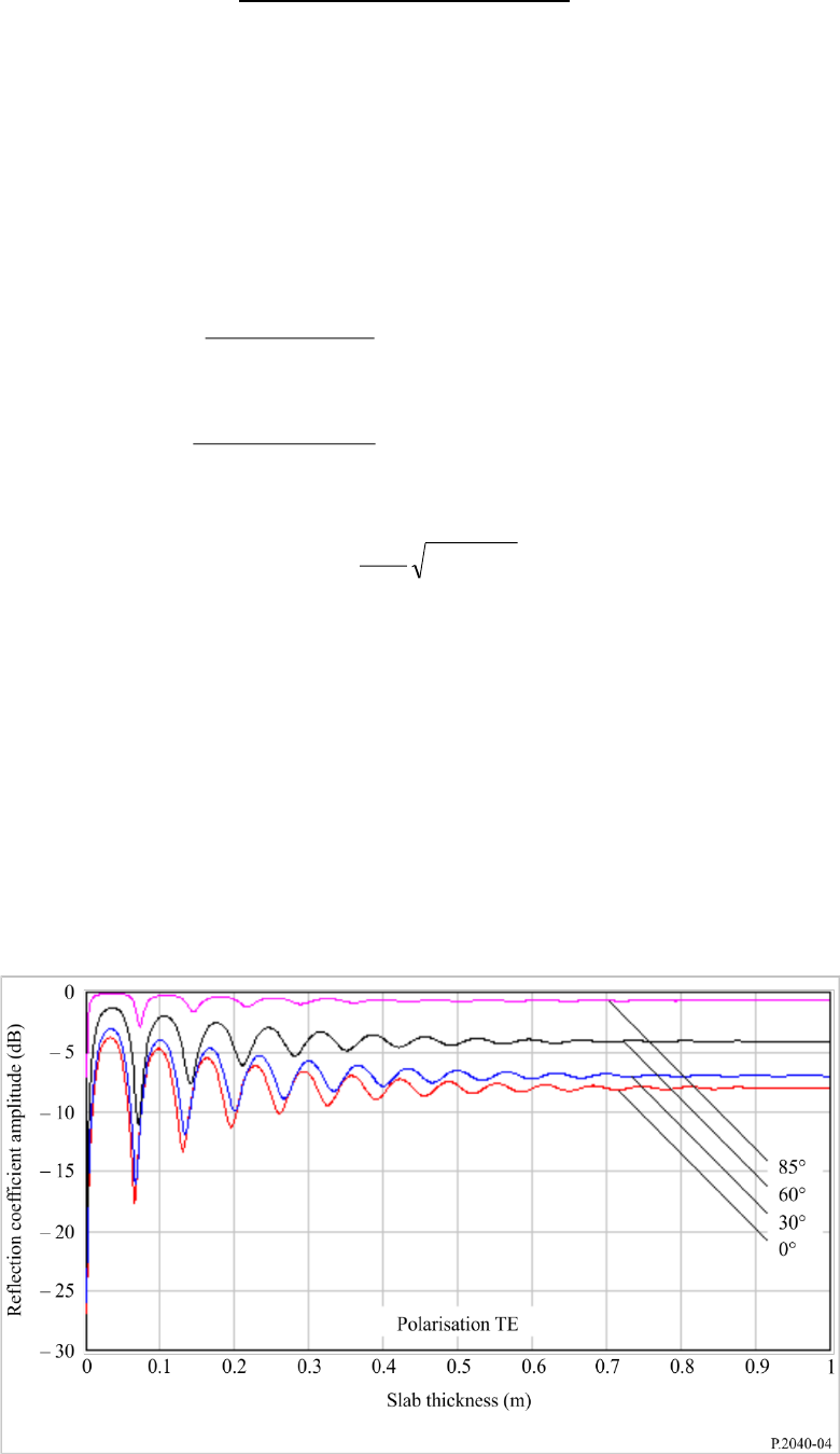
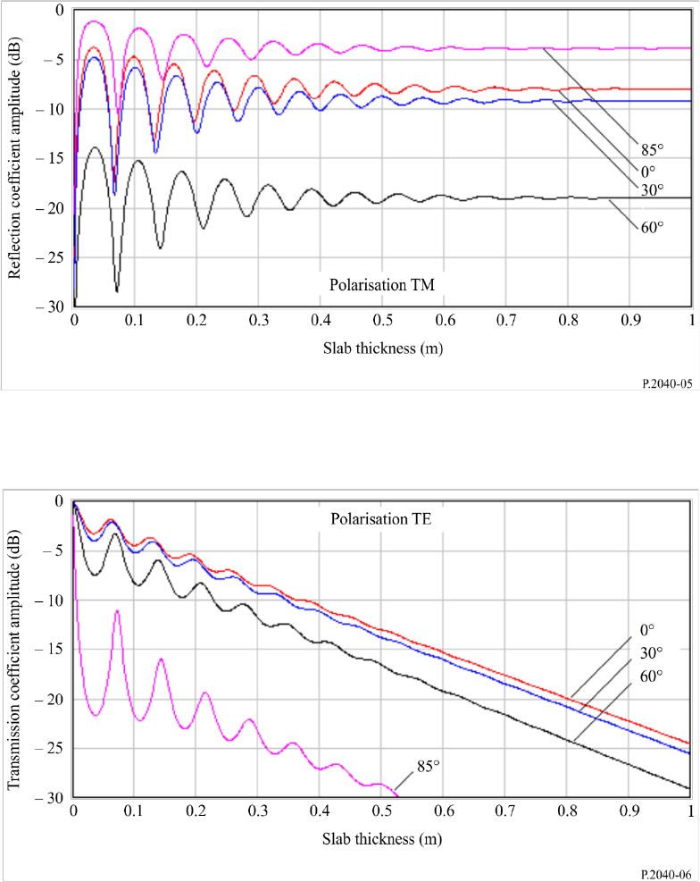
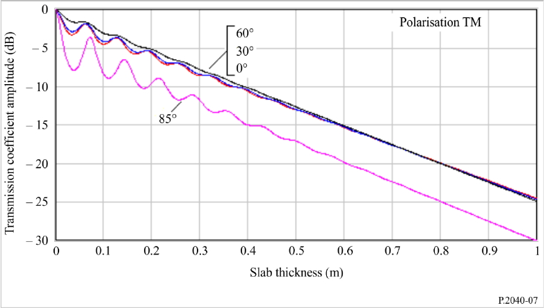
2.2.2.3 Calculation examples
Figures 4 to 7 show examples of results from equation (42a) for a single concrete slab at 1 GHz with
four incidence angles. The same results may be obtained from equations (43a) and (43b). The
electrical properties for concrete are taken from Table 3.
FIGURE 4
Reflection coefficient for a concrete slab at 1 GHz, TE polarisation
Rec. ITU-R P.2040-3 15
FIGURE 5
Reflection coefficient for a concrete slab at 1 GHz, TM polarisation
FIGURE 6
Transmission coefficient for a concrete slab at 1 GHz, TE polarisation
16 Rec. ITU-R P.2040-3
FIGURE 7
Transmission coefficient for a concrete slab at 1 GHz, TM polarisation
It will be noted in Figs 5 and 7 that the coefficients for TM polarization for 85 degrees incidence have
anomalous values compared to the ordering of the other three angles. This is the effect of the
minimum in reflection coefficient visible in Fig. 2 for TM polarization, known as the
pseudo-Brewster angle.
2.2.3 Waveguide propagation in buildings
2.2.3.1 Theory on frequency characteristics of attenuation constant in waveguide
A waveguide may comprise of a hollow space surrounded by lossy dielectric materials. In the case of
a building structure, a corridor, underground mall, or tunnel can be considered as a waveguide. The
radiowave power that propagates in a waveguide is attenuated according to the distance. It is well
known that a waveguide has frequency characteristics such as the cut-off frequency that varies
according to the shape. In this section, a formula is presented to derive the attenuation constant for
the frequency characteristics in a waveguide.
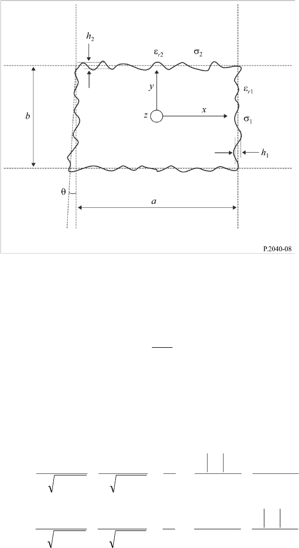
The cross-section of a square waveguide structure is shown in Fig. 8. In this case, the intrinsic constants
of the lossy dielectric material are different for the sidewalls and for the ceiling and the floor.
Rec. ITU-R P.2040-3 17
FIGURE 8
Cross-section of waveguide and material constants
In Fig. 8, a is the width and b is the height of the waveguide (m), h
1
and h
2
are the root mean square
roughness of the Gaussian distribution of the surface level, and is the tilt of the root mean square
(rad). The complex permittivity values for materials
ri
*
are calculated as follows.
2,1,
0
"*
=
+−= ij
i
ri
ri
ri
(45)
where
ri
is the relative dielectric constant and
i
is the conductivity. The quantity
ri
″ is the loss
tangent of the materials, is the angular frequency and
0
is the permittivity of free space.
The basic attenuation constant is formulated as follows.
( ) ( )
( ) ( )
−
+
−
−
−
+
−
=
−
+
−
−
−
+
−
=
11
1
Im
2
11
1
ReK
1
1
1
Im
2
1
1
1
ReK
*
2
4
2
*
2
*
1
4
*
2
3
2
*
1
3
2
v,
*
2
4
*
1
4
2
*
1
*
2
3
*
1
3
1
2
h,
*
*
r
r
r
r
r
r
vbasic
rr
r
rr
r
hbasic
ba
ba
L
ba
ba
L
(dB/m) (46)
K
h
and K
v
are constant values that are dependent on the section shape. The constant values dependent
on the section shape are given in Table 1.
18 Rec. ITU-R P.2040-3
TABLE 1
Constant values for various cross-section shapes
Shape
Circle
Ellipse
Square
Arch-backed
K
h
5.09
4.45
4.34
5.13
K
v
5.09
4.40
4.34
5.09
The formulas mentioned above are valid based on equation (47) representing the condition of
constraint.
(m) (47)
Unique characteristics in square shape case
The attenuation constant due to roughness, which is regarded as local variations in the level of the
surface relative to the mean level of the surface of a wall, is given by:
+
=
+
=
2
2
2
2
2
1
2
v,
2
2
2
2
2
1
2
h,
K
K
b
h
a
h
L
b
h
a
h
L
vroughness
hroughness
(dB/m) (48)
The attenuation constant due to the wall tilt is given by:
=
=
22
v,
22
h,
K
K
vtilt
htilt
L
L
(dB/m) (49)
Therefore, the total attenuation constant in a square shape case is the sum of the above losses:
(dB/m) (50)
2.2.3.2 Applicability of waveguide theory
The waveguide theory shows good agreement with the measured propagation characteristics in the
corridor in the frequency range of 200 MHz to 12 GHz in case there is no pedestrian traffic in the
corridor.
1
1
2
1
1
−
−
r
r
r
b
a
vtiltvroughness
v
basicv
htilthroughness
h
basich
LLLL
LLLL
,,,
,,,
++=
++=
Rec. ITU-R P.2040-3 19
Effect of pedestrian traffic on waveguide
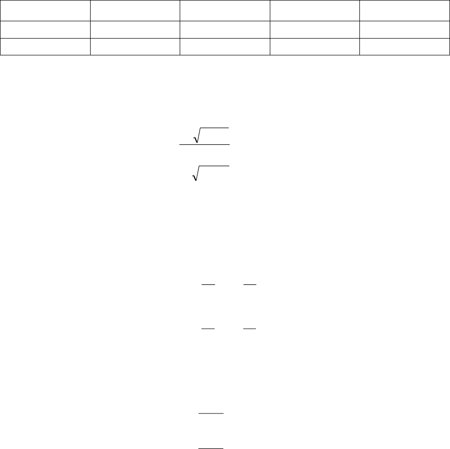
Figure 9 shows a comparison of the theoretical and measured attenuation constant values during the
day (when pedestrian traffic is present), and during the night (when the corridor is empty). Theoretical
values are calculated based on the parameters given in Table 2.
TABLE 2
Parameters used in underground calculation
Width
(m)
Height
(m)
Tilt
(degrees)
Roughness
Material constant
h
1
h
2
r1
r2
Underground
6.4
3.0
0.35
0.4
0.2
15
10
0.5
0.1
FIGURE 9
Attenuation constant comparison for day and night
Figure 9 shows that the waveguide theory is applicable to realistic propagation characteristics in the
corridor in the frequency range of 200 MHz to 12 GHz at night. However, the waveguide theory is
not applicable to realistic propagation characteristics during daytime, because the received power is
attenuated by pedestrian traffic.
Therefore, the waveguide theory is applicable to situations where there is no influence from
shadowing obstacles.
2.3 Theory and results for frequency selective surface materials
2.3.1 Frequency selective surfaces
The power of scattering waves varies with roughness of surfaces. In this section, a theory for
calculating scattered fields from the surface having round convexity array is described. First, for
parameterizing the roughness of the surface, the rough surface is defined by using a round convexity
array formed by locating circular cylinders periodically.
20 Rec. ITU-R P.2040-3
Second, the reflection coefficient of the scattered fields is defined by using the lattice sums
characterizing a periodic arrangement of scatterers and the T-matrix for a circular cylinder array.
Third, a numerical result that shows the frequency-depending characteristic of the reflection from the
round convexity’s surface is shown. Finally, a measurement result is shown to explain that the power
of scattering waves varies with the frequency of an incident wave when there is a round convexity
array on the surface of a building.
2.3.2 Theory for wave propagation around the surface of round convexity array
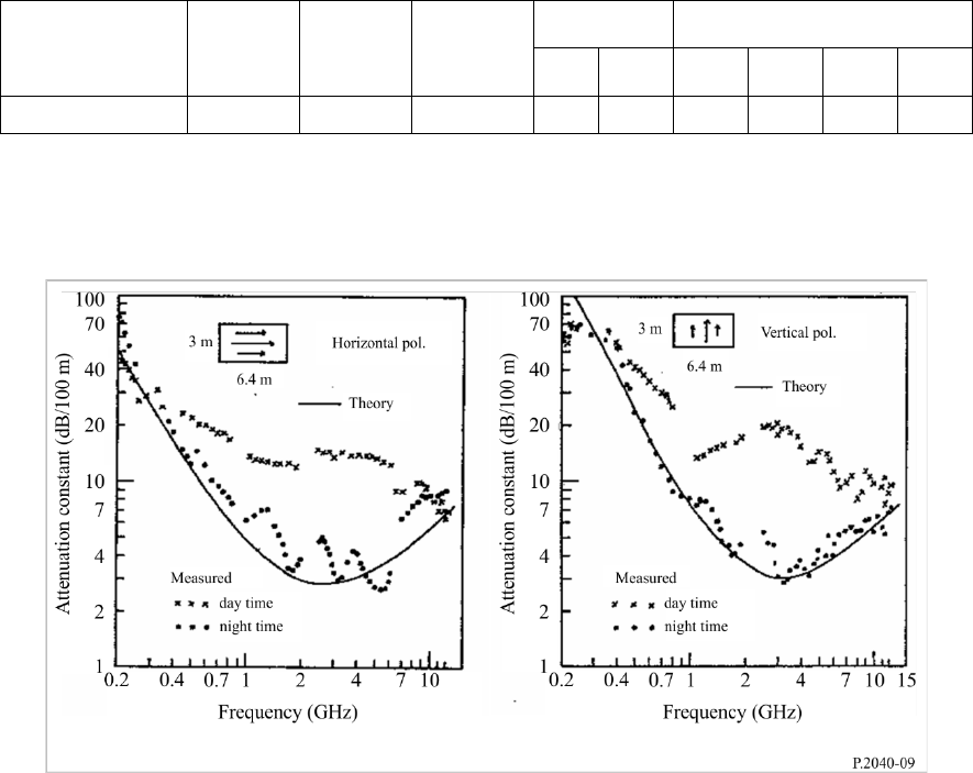
By making periodical round convexity array on a surface of a building, as shown in Fig. 10,
reflection/scattering waves can be controlled larger than those from the flat surface. The theory to
calculate the scattered waves from the periodic arrays of circular cylinders can be used to define the
propagation waves around a convexity array of a surface.
FIGURE 10
The surface of round convexity array
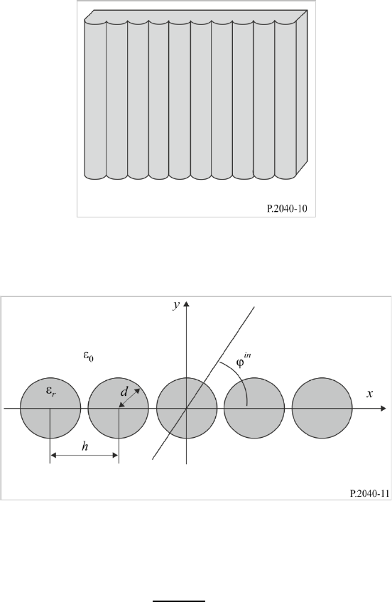
FIGURE 11
Geometry of a periodic array of circular cylinders
When the identical circular cylinders are situated periodically in an x axis as shown in Fig. 11, the
power reflection coefficient R
for the
-th propagating mode with k
> 0 is given as:
in
(51)

Rec. ITU-R P.2040-3 21
where k
0
= 2
0
,
0
is the wavelength of the waves indenting in angle
in
. In equation (51),
and
are obtained as follows:
(52)
(53)
where
is the unit matrix,
,
and h is the periodic space
between each round convex.
is a square matrix whose elements are defined in terms of the following
lattice sums:
in
in
(54)
where
is the m-th order Hankel function of the first kind.
is the T-matrix for the scattered fields
and is given by the following diagonal matrix for the incident electric field
and the incident
magnetic field
, respectively.
(55a)
(55b)
where
is the relative permittivity of the dielectric cylinder,
is the m-th order Bessel function,
the prime demotes the derivative with respect to the argument, and
denotes the Kronecker’s delta.
denotes a column vector whose elements represent unknown amplitudes of the incident field.
in
(56)
2.3.3 Calculation results
The calculation result of a power reflection coefficient is shown in Fig. 12. The result is calculated
by using equation (51) in the case that the electric field
is transmitted in the angle
in
= 90° to the
dielectric round convexities whose diameter and permittivity are d = 0.3h and
r
= 2.0, respectively.
In the result, there is the frequency band that the incident wave is reflected almost completely by the
surface even if its material is a lossless dielectric substance.
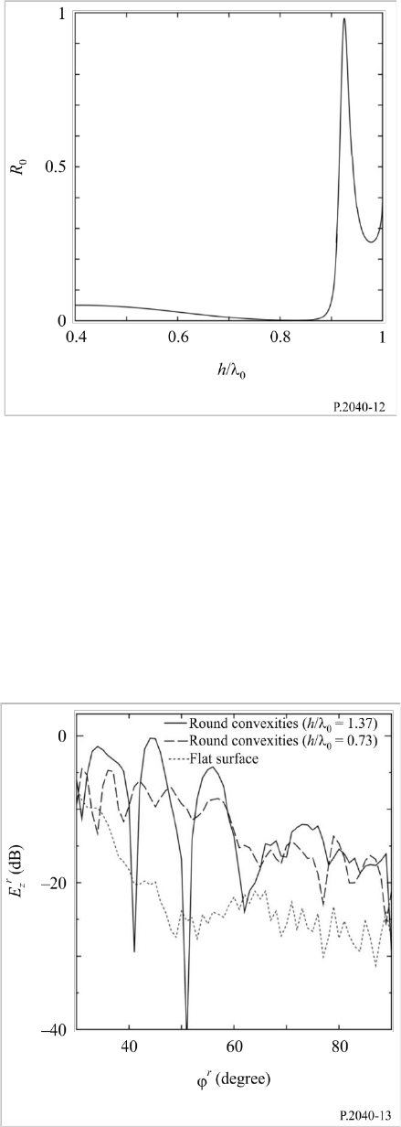
22 Rec. ITU-R P.2040-3
FIGURE 12
Power reflection coefficient
R
0
as functions of the normalized wavelength
h
/
0
at normal incidence electric field
2.3.4 Measurement
The measurements of the scattered waves from the building having the round convexity array were
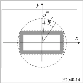
carried out. Figure 13 shows the comparison of the scattered waves from the building between the
flat surface and the surface with round convexity arrays. The scattered waves from the building were
measured in various reflected angles
r
between 30° to 90°, when the electric field is transmitted in
the angle
in
. The incident angle and reflection angle are defined as shown in Fig. 14.
FIGURE 13
Geometry of a periodic array of circular cylinders
Rec. ITU-R P.2040-3 23
FIGURE 14
A plane figure of the compositional diagram
for measurements
The measurement results show that the power of the scattered field from the surface having a round
convexity array becomes larger than that from the flat surface, and can be controlled by the period
between and diameter of each round convexity. Note that the relative permittivity and the conductivity
of the building material were estimated as
r
= 6.0 and σ = 0.1 S/m, respectively.
3 Compilations of electrical properties of materials
Representative data on material electrical properties can be hard to find, as characteristics are
expressed using different combination of parameters, and the relative permittivity may be quoted at
frequencies that are not close to that of interest. A table of representative material properties has
therefore been compiled using the curve-fitting approach described in § 2.1.4.
Data from eight sets of material electrical properties (a total of more than 90 separate characteristics)
given in the open literature have been collated, converted to a standard format and grouped into
material categories.
For each group, simple expressions for the frequency-dependent values of the real part of the relative
permittivity, ', and the conductivity, , were derived. These are:
(57)
and:
(58)
where f is frequency in GHz and is in S/m. (' is dimensionless.) The values of a, b, c and d are
given in Table 3. Where the value of b or d is zero the corresponding value of
or is a or c
respectively, and independent of frequency.
If required, the imaginary part of the relative permittivity " can be obtained from the conductivity
and frequency:
f/98.17 =
(59)
Parameters for air, metal and three conditions of ground are included in Table 3 for completeness.

24 Rec. ITU-R P.2040-3
TABLE 3
Material properties
Material class
Real part of relative
permittivity
Conductivity
S/m
Frequency range
a
b
c
d
GHz
Vacuum (≈ air)
1
0
0
0
0.001-100
Concrete
5.24
0
0.0462
0.7822
1-100
Brick
3.91
0
0.0238
0.16
1-40
Plasterboard
2.73
0
0.0085
0.9395
1-100
Wood
1.99
0
0.0047
1.0718
0.001-100
Glass
6.31
0
0.0036
1.3394
0.1-100
Glass
5.79
0
0.0004
1.658
220-450
Ceiling board
1.48
0
0.0011
1.0750
1-100
Ceiling board
1.52
0
0.0029
1.029
220-450
Chipboard
2.58
0
0.0217
0.7800
1-100
Plywood
2.71
0
0.33
0
1-40
Marble
7.074
0
0.0055
0.9262
1-60
Floorboard
3.66
0
0.0044
1.3515
50-100
Metal
1
0
10
7
0
1-100
Very dry ground
3
0
0.00015
2.52
1-10 only
Medium dry ground
15
−0.1
0.035
1.63
1-10 only
Wet ground
30
−0.4
0.15
1.30
1-10 only
The frequency ranges given in Table 3 are not hard limits but are indicative of the measurements used
to derive the models. The exceptions are the three ground types where the 1-10 GHz frequency limits
must not be exceeded. Typical values of relative permittivity and conductivity for different types of
ground, as function of frequency in the range 0.01 MHz to 100 GHz, are given in Recommendation
ITU-R P.527.
The loss tangents of all the dielectric materials in Table 3 are less than 0.5 over the frequency ranges
specified. The dielectric limit approximations for the attenuation rate given in equations (24) and (27)
can therefore be used to estimate the attenuation of an electromagnetic wave through the materials.
Rec. ITU-R P.2040-3 25
Attachment 1
to Annex 1
Alternative method to obtain reflection and transmission coefficients
for building materials represented by N dielectric slabs
based on ABCD matrix formulation
An alternative formulation of the method in § 2.2.2.1 is given below to obtain the reflection, R, and
transmission, T, coefficients for a building material represented by N dielectric slabs based on the
ABCD matrix formulation, as illustrated in Fig. 5. The regions on both sides of the building material
are assumed to be free space. This alternative method produces exactly the same results as that given
in § 2.2.2.1.
00
00
2 CZZBA
CZZB
R
++
−
=
(60a)
(60b)
where A, B and C are the elements of the ABCD matrix given, using matrix multiplication, by:
(61a)
where:
(61b)
(61c)
(61d)
(61e)
2/1
0
2
sin
–1)(cos
==
m
mmmm
kk
(61f)
=
2
0
k
(61g)
mm
kk =
0
(61h)
is the free-space wavelength, k
0
is the free-space wave number,
m
and k
m
are the complex relative
permittivity and wave number in the m-th slab,
m
is the propagation constant in the direction
perpendicular to the slab plane, and d
m
is the width of the m-th slab.
The wave impedances Z are given, according to incidence polarization, by:
TE polarisation (62a)
TM polarisation (62b)
where:
(63a)
=
NN
NN
mm
mm
DC
BA
DC
BA
DC
BA
DC
BA
......
11
11

26 Rec. ITU-R P.2040-3
(63b)
(63c)
The wave impedance
in equation (63c) is the free space impedance, and it can be obtained from
equations (62a) and (62b) through setting
.
